Toolbox Chaos practical guide
System Catalog
Navigate 38 registered examples, recognize model families and supported dimensions, and choose a system that matches the question you want to investigate.
Objective
What you will accomplish
Select an appropriate registered system without treating its catalog label or default parameters as a new scientific conclusion.
Before you begin
- Know whether your question concerns continuous time, discrete iteration, delay dynamics, or comparison across model families.
- Consult the cited source for a model before using its equations or parameters in a publication.
Reference outputs
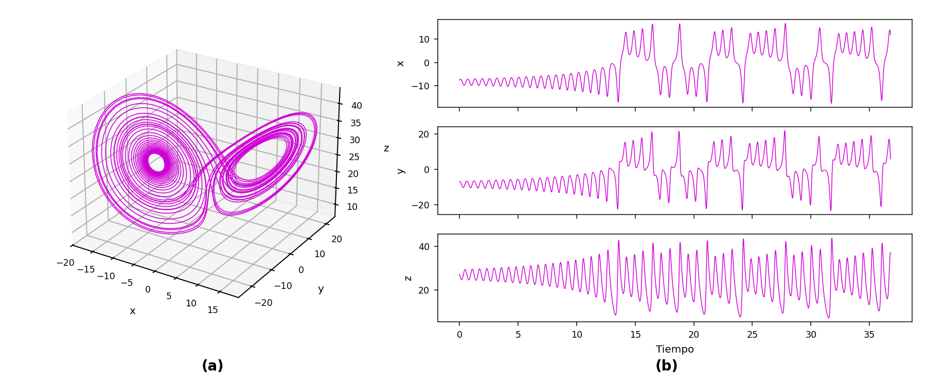
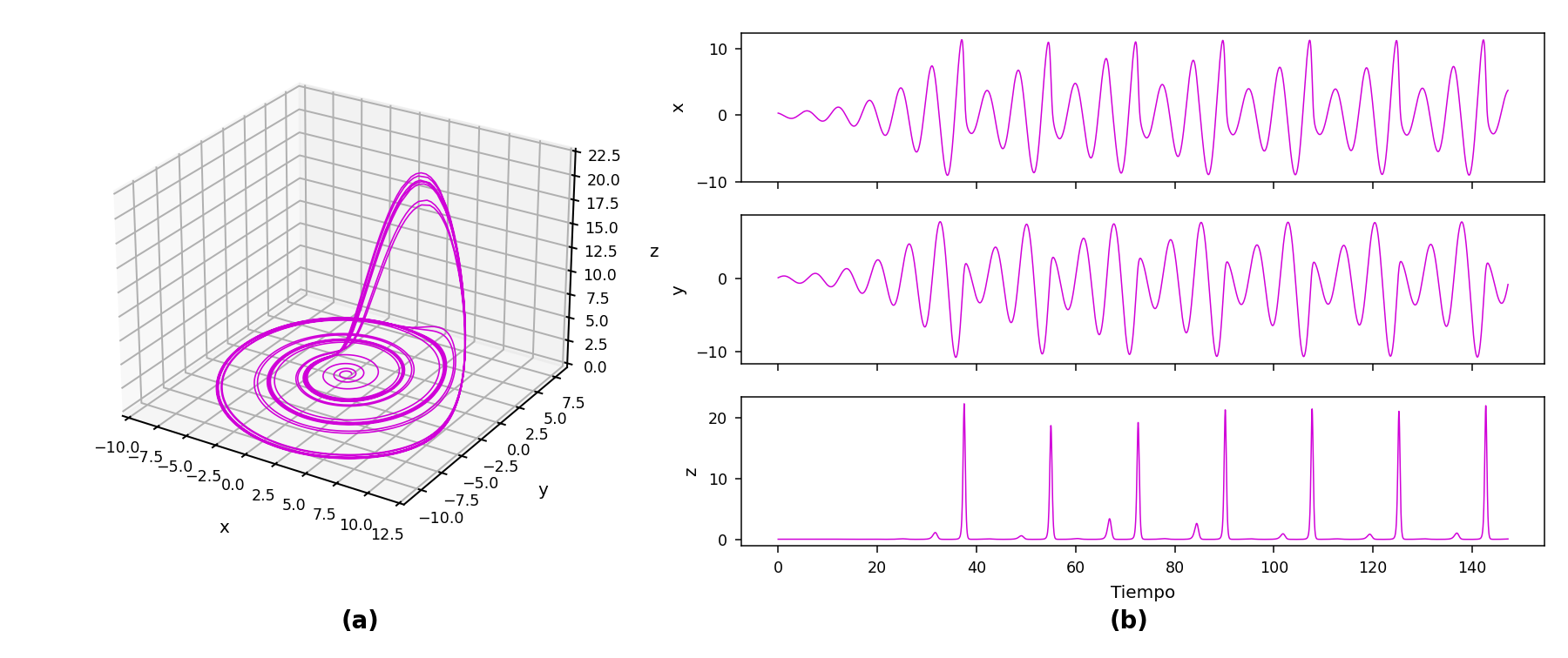
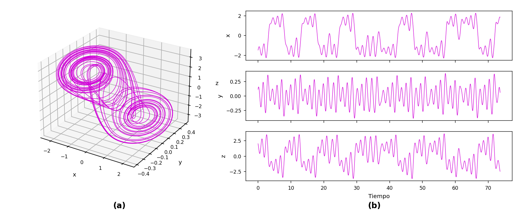
What these views can show
Procedure
Step-by-step workflow
-
Choose the model family
Use an ODE flow when step size and physical or nondimensional time are central. Use a map when the state advances by iterations. Treat Mackey–Glass as a delay-model workflow rather than an ordinary three-state ODE.
Lorenz-96 and the four-dimensional hyperchaotic Lorenz example have display-specific considerations; inspect the interface response after selection.
-
Read the populated metadata
After selecting a system, read the parameter labels in their displayed order, the initial-state labels, default values, and dimension-dependent controls.
Do not transfer a parameter vector from one model to another merely because both use letters such as a, b, or c.
-
Run the registered baseline
Generate a portrait and time series using the preset before changing a parameter. Save this baseline as the reference for later comparisons.
Check boundedness and transient behavior. A preset is an entry point for exploration, not a guarantee that every horizon and step reproduces a textbook figure.
-
Vary one declared input
Change one parameter or one initial-state component while keeping the method, step, and horizon fixed. Use a structured series rather than opportunistic trial and error.
If the question is about a broad interval, move to Bifurcación or a documented research workflow instead of collecting isolated screenshots.
-
Check feature compatibility
The 3D view requires a three-state display, analytical or numerical equilibria are restricted to supported ODE flows, and Lyapunov uses its stated 3D ODE-flow contract.
Basin and coexistence panels depend on registered cases or destination rules; availability in the system selector does not imply every tab supports that model.
Registered model groups
The current selector contains 38 implemented entries. The grouping below is for navigation; the GUI remains the authority for the exact parameter order and defaults.
- Continuous three-state examples: Lorenz, Rössler, Chua / double scroll, Chen, Wang–Chen with variable equilibria, Nazarimehr with a line of equilibria, Lü, Duffing–Ueda, Rabinovich–Fabrikant, Rikitake, Unified Lorenz–Chen, Thomas / labyrinth, and Hindmarsh–Rose.
- Discrete maps: Hénon, logistic, and Ikeda.
- Delay and special displays: Mackey–Glass, Lorenz-96, and the four-dimensional hyperchaotic Lorenz model.
- Classic compact flows: Sprott A through Sprott S, nineteen separate catalog entries.
Choosing by research question
- Sensitivity and phase-space teaching: begin with Lorenz or Rössler.
- Discrete iteration and period-doubling: begin with the logistic or Hénon map.
- Circuit-inspired piecewise dynamics: use Chua and preserve its parameter convention.
- Slow–fast or bursting behavior: inspect Hindmarsh–Rose through time series before geometric projections.
- High-dimensional or delay behavior: state explicitly which variables or embedding are displayed; a 3D picture is not the complete state space.
Result
Expected output
- A baseline run whose system type, parameter order, state dimension, initial condition, and numerical settings are all recorded.
- A defensible reason for selecting the model and the tabs used to study it.
Interpretation
How to read it
The catalog organizes implemented examples and supplies operational defaults. It does not certify that a generated orbit is chaotic, attracting, unique, or hidden.
Comparisons across systems are meaningful only when the numerical resolution, discarded transient, observed duration, and plotted variables are made explicit.
Export
Reproducibility checklist
- Use the full catalog label and cite the scientific source for the equations.
- Record flow, map, delay, or special-display status and the variables actually plotted.
- Keep the untouched preset result alongside parameter-modified results.
Applications
Where this workflow helps
- Comparative teaching examples for continuous and discrete dynamics.
- Benchmarking numerical methods across different nonlinear vector fields.
- Selecting candidate models for parameter, spectral, stability, or multistability studies.
Limits
What it does not establish
- A catalog entry is an implemented model, not an exhaustive validation of all parameter regimes.
- Sprott A–S catalog flows are distinct from the separate Explorador Sprott code and local-dictionary workflow.
- Published descriptions involving hidden dynamics must not be reinterpreted as a Toolbox Chaos localization result.