Toolbox Chaos practical guide
Interface Overview
Map each question to the correct tab, understand shared trajectories, and keep model, numerical, and visual controls conceptually separate.
Objective
What you will accomplish
Learn the complete GUI workflow before beginning a long simulation or parameter campaign.
Before you begin
- Open Toolbox Chaos and maximize the window so the tab row and status area are visible.
- Know the difference between a dynamical-system parameter, an initial condition, and a numerical integration setting.
Reference outputs
What these views can show
Procedure
Step-by-step workflow
-
Identify the repeated control pattern
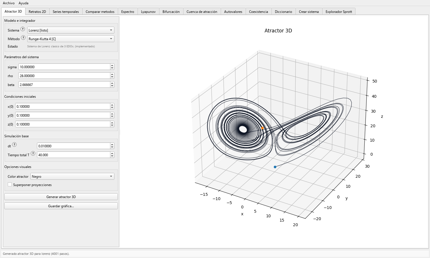
Most numerical tabs place controls on the left and results on the right. Start by selecting a system; the interface then updates parameter labels and state dimension.
Where present, method, step, and duration controls specify the numerical experiment. Color, projection, and axis controls change presentation rather than the model equations.
-
Start from a primary trajectory
Atractor 3D, Retratos 2D, Series temporales, and Espectro can run a local simulation. The first three also establish the trajectory used by compatible reuse actions.
When pressing Usar última trayectoria, confirm that the selected system matches the system associated with the stored trajectory.
-
Move from views to diagnostics
Use Comparar métodos for numerical sensitivity, Espectro for Welch PSD or amplitude spectrum, Lyapunov for the supported finite-time ODE-flow calculation, and Autovalores for supported equilibrium analysis.
Use Bifurcación, Cuenca de atracción, and Coexistencia for structured parameter or initial-condition exploration rather than for a single portrait.
-
Use learning and model tools deliberately
Diccionario connects terminology to the visual workflows. Crear sistema validates and simulates user-defined flows or maps. Explorador Sprott provides its own code, search, gallery, and local-dictionary workflow.
A model created or loaded by the user is not automatically part of the curated catalog and does not inherit catalog-specific equilibrium or basin support.
-
Read status and error messages
Do not dismiss warnings about dimension, incompatible shared trajectories, unsupported system type, transient length, or invalid definitions. They are part of the numerical contract.
If a run fails, reduce the experiment to a catalog preset and known method before changing several inputs at once.
-
Use the application menus
Open Archivo → Abrir carpeta de resultados to reach the user output location without guessing a path.
Use Ayuda for the bundled local documentation, citation information, and About panel when recording the software identity used in a study.
The 13 tabs at a glance
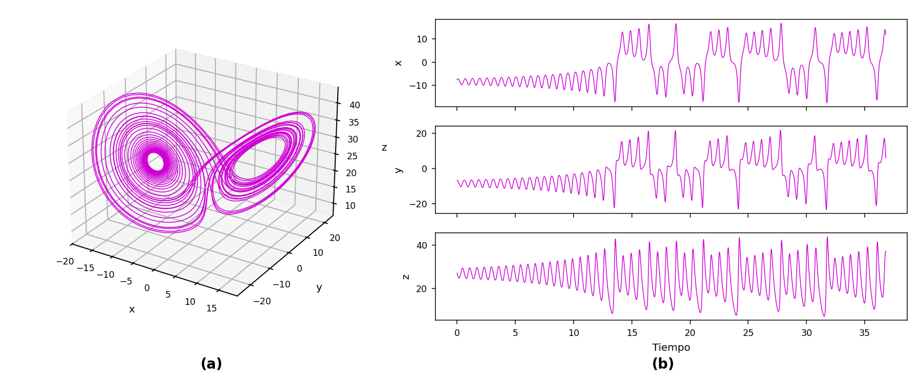
- Atractor 3D — three-state geometry, optional coordinate-plane projections, and figure export.
- Retratos 2D — selectable pairwise projections with a shared-trajectory option.
- Series temporales — one state history per displayed variable with independent colors.
- Comparar métodos — Euler, Heun, and RK4 under one common setup.
- Espectro — Welch power spectral density or a one-sided amplitude spectrum.
- Lyapunov — supported finite-time QR–Benettin spectrum for integer-order 3D ODE flows.
- Bifurcación — parameter sweeps with model-aware controls and optional supported constructions.
- Cuenca de atracción — finite grids of initial conditions classified by a supported destination rule.
- Autovalores — supported ODE equilibria, Jacobian eigenvalues, and local classification.
- Coexistencia — registered cases compared at common parameters and different starts.
- Diccionario — local conceptual reference.
- Crear sistema — safe no-code definitions, validation, simulation, and JSON exchange.
- Explorador Sprott — code decoding, synthetic exploration, local user-owned dictionaries, examples, and gallery export.
- Archivo and Ayuda menus — results folder, local documentation, citation details, and application identity.
Result
Expected output
- You can name the tab that answers a particular research question and state which settings affect the model, numerical solution, or appearance.
- You can reuse a computed trajectory without silently switching systems or recomputing with different settings.
Interpretation
How to read it
The tabs form an evidence ladder: trajectory views reveal finite behavior, diagnostics quantify selected properties, and sweeps compare behavior across a declared grid. No single tab replaces the others.
A visually persuasive plot may still depend strongly on the step, duration, discarded transient, and initial state. Treat the status line and saved settings as part of the result.
Export
Reproducibility checklist
- Export from the tab that produced the final evidence rather than capturing an arbitrary screen crop.
- Record the tab name and whether it simulated locally or reused the last trajectory.
- For multi-tab studies, use one run identifier across figures and notes.
Applications
Where this workflow helps
- Designing a classroom sequence from portraits to quantitative diagnostics.
- Planning a research exploration so each question has an explicit GUI operation and output.
- Training a team to use consistent numerical and naming conventions.
Limits
What it does not establish
- Not every diagnostic supports every model type or dimension; the interface reports these compatibility boundaries.
- Shared trajectories improve consistency but do not automatically preserve every display choice or explanatory note.
- The GUI supports simulation, visualization, and parameter exploration; it is not a hidden-attractor localization interface.