About
Project metadata, archive reference, and build baseline.
Key Features
Desktop tools for simulation, visual analysis, and reproducible figure generation.
Concept-first toolbox
Learning Chaos With Figures
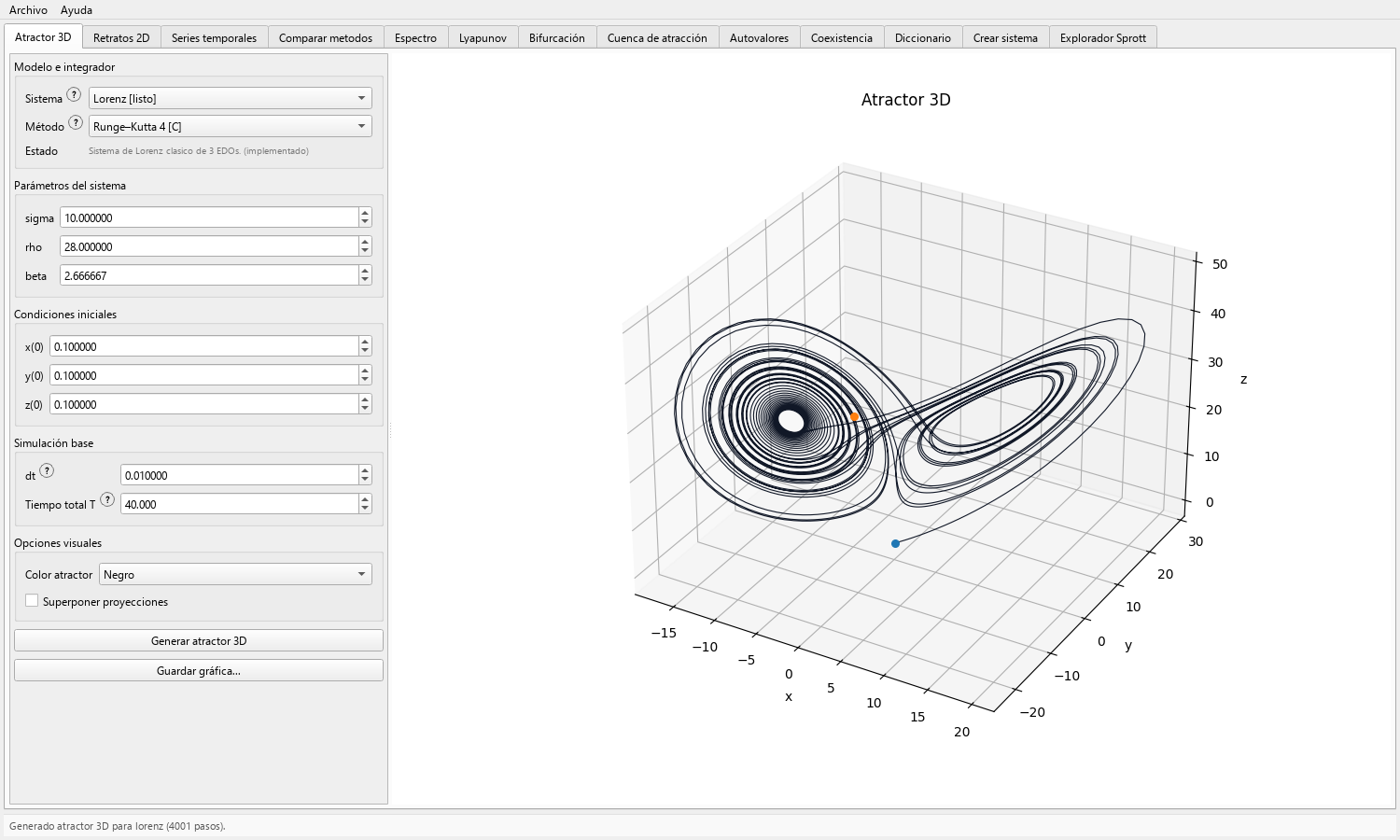
Toolbox Chaos is organized around the same teaching idea as the dictionary PDF: students learn faster when each concept is tied to a concrete graph. The overview shows the available workflows; the documentation explains how to read each graph in detail.
Read the visual theory primer ->Theory Through Graphics
The dictionary and web documentation connect definitions with reproducible figures, so students can read what each diagnostic is actually showing.
Separate Visual Tasks
A basin map, a coexistence comparison, a bifurcation diagram, and a Lyapunov plot answer different questions. The site keeps those workflows separated.
Reproducible Examples
Examples use explicit systems, parameters, initial conditions, projection choices, and retained windows so students can reproduce the plots.
Compact-system exploration workflow
Sprott Explorer
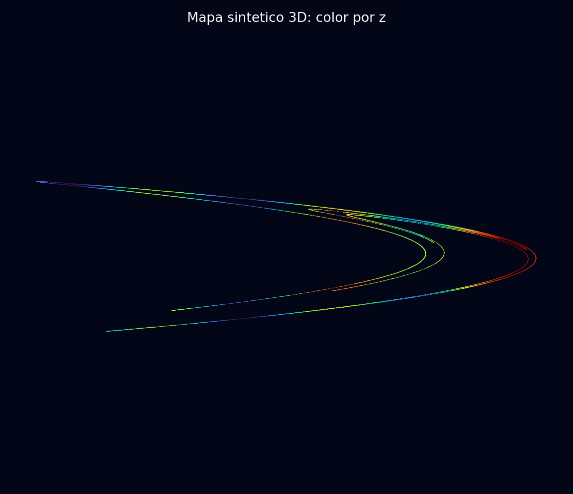
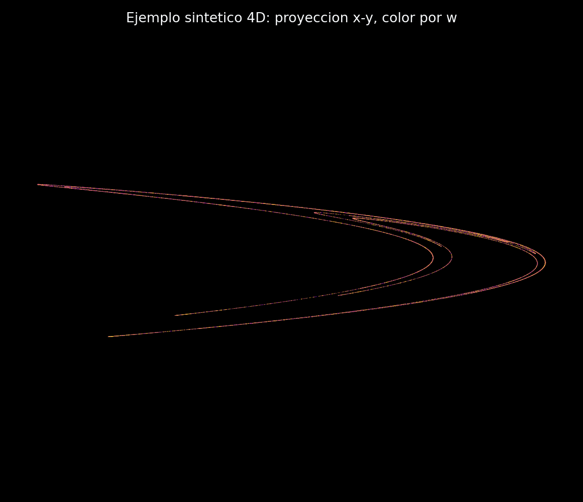
The Sprott Explorer invites students to experiment with compact dynamical-system recipes inspired by J. C. Sprott's strange-attractor work. Load a generated example, change the projection or visual preset, and watch how a short code becomes a map, a flow, or a dense phase-space object worth investigating.
The public page uses reproducible educational examples, while the documentation explains the decoding logic, search filters, plotting choices, and parameter effects.
Open the Sprott guide ->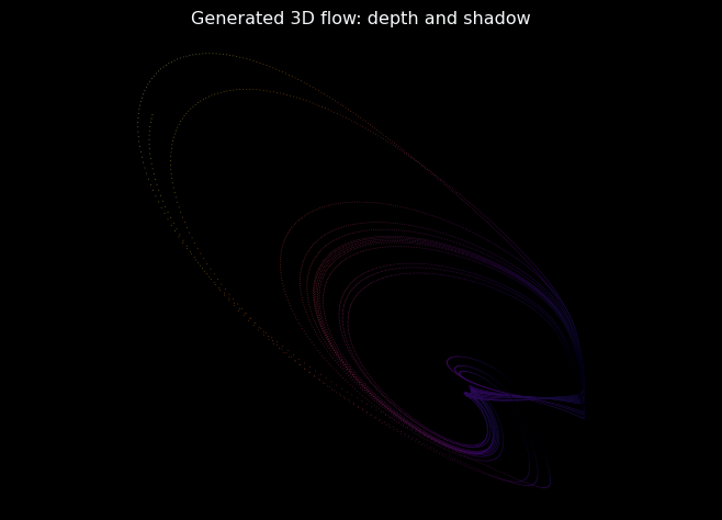
Working Pattern
A practical loop for moving from a first run to a figure worth saving.
Choose a scientific question
Start from the view or comparison you need: trajectory geometry, time evolution, integration method, spectrum, bifurcation, basin, coexistence, or local stability.
Load a coherent preset
Use a registered system so equations, parameters, initial state, and integration scale begin in a known range.
Run a low-cost pass
Use coarse grids, shorter sweeps, or fewer points to check whether the selected region is meaningful.
Refine one control
Change one value at a time: time step, total time, transient, parameter range, projection, or density.
Compare complementary evidence
Use geometry, time series, method comparison, spectra, eigenvalues, basins, bifurcation, and Lyapunov estimates for distinct questions.
Record and export
Save the system, parameters, initial conditions, method, step, transient, and figure or data artifact needed to reproduce the run.
Practical Guides
The complete guide set covers installation, every major GUI workflow, figures, exports, research applications, and responsible interpretation.
Getting Started
Install the desktop application, run a first catalog example, reuse its trajectory, and save a figure.
Interface Overview
Understand the 13 tabs, shared trajectory workflow, controls, status messages, and where each task belongs.
System Catalog
Choose among 38 registered flows, maps, delay and special models without confusing catalog status with a dynamical claim.
Concepts and Visual Theory of Chaos
Definitions, figures, and reading strategies for students entering chaotic systems for the first time.
Lorenz Attractor Quick Start
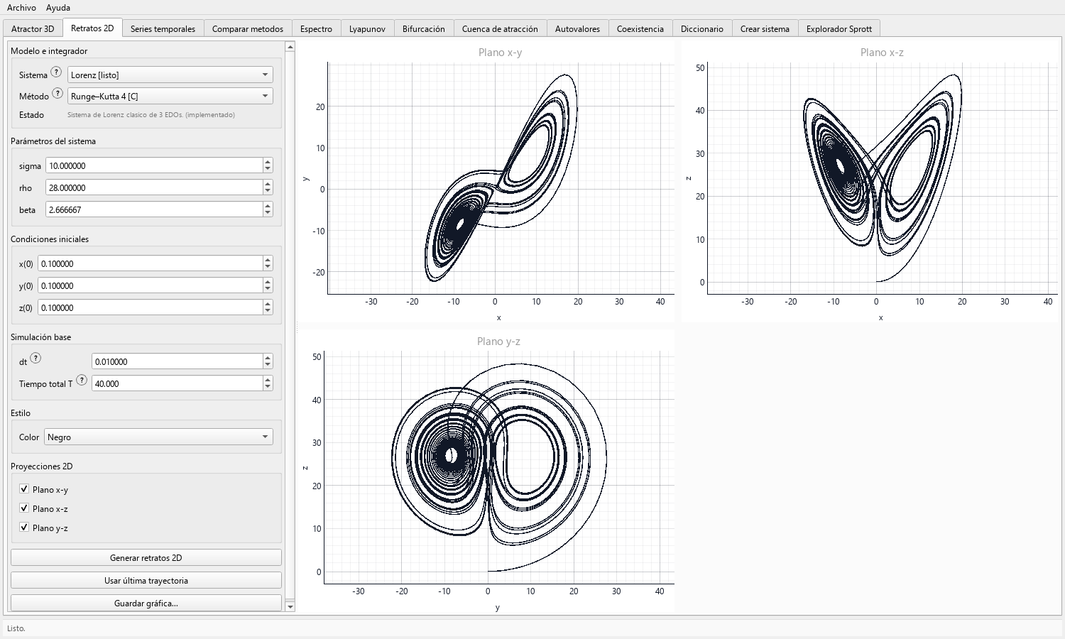
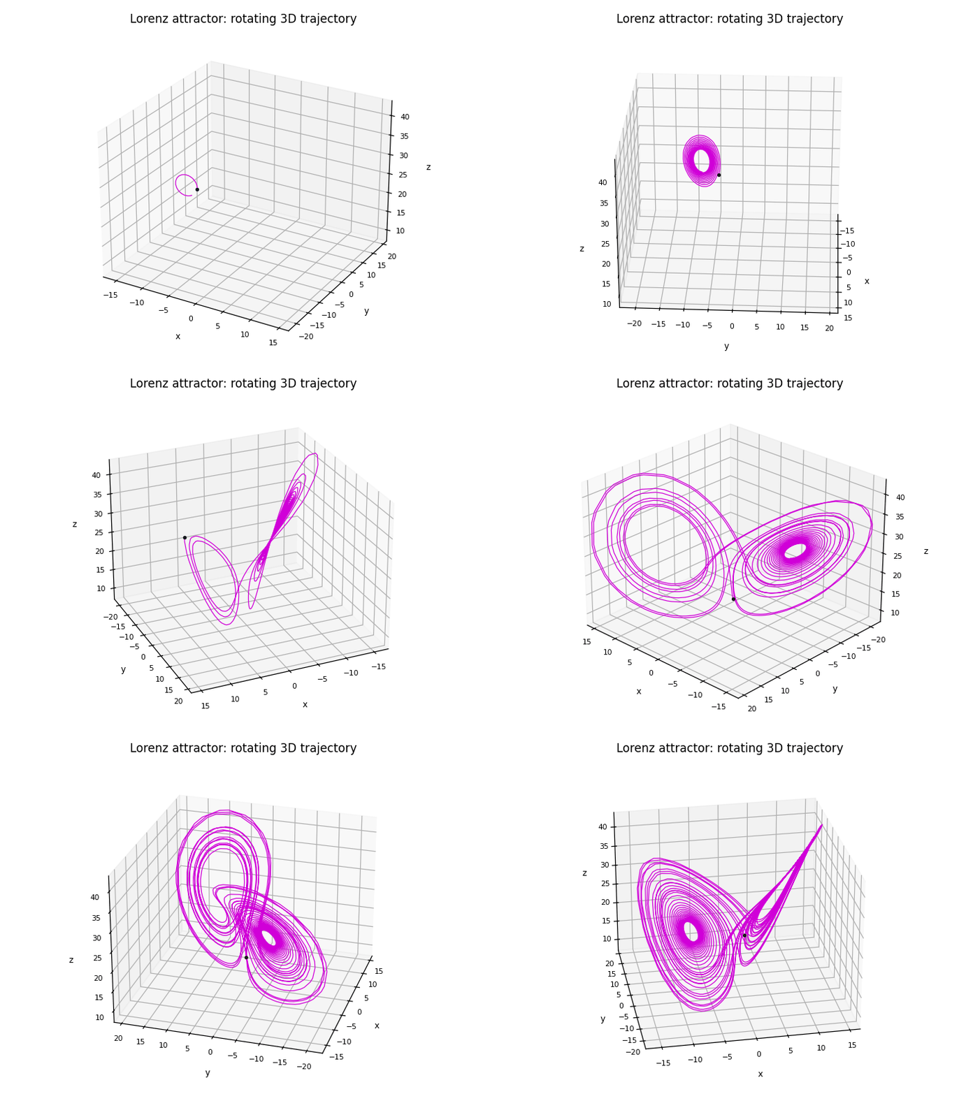
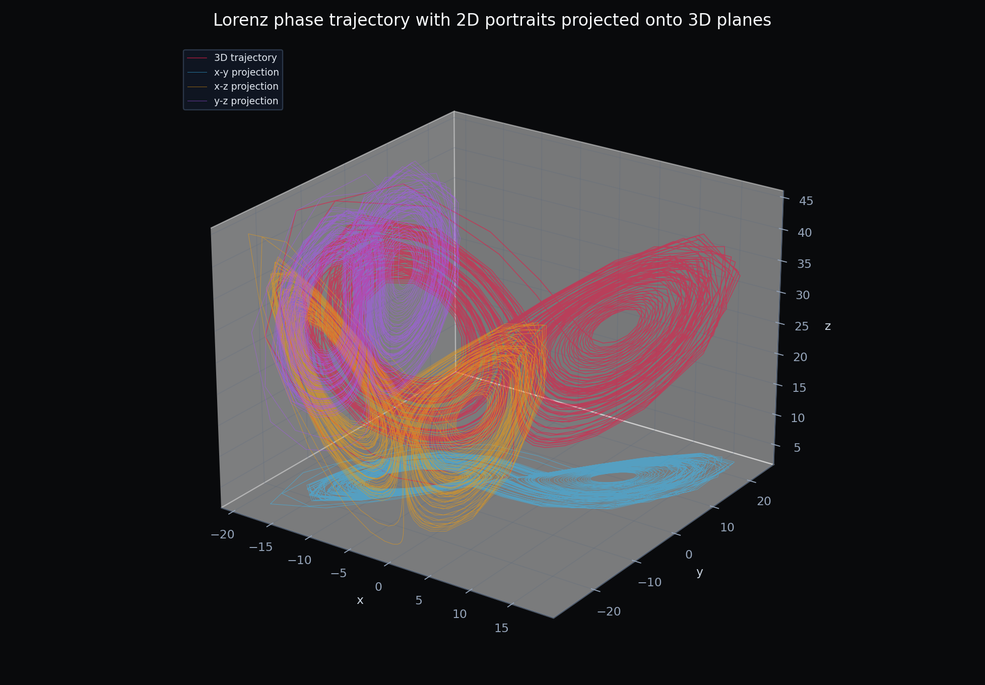
Set parameters, run a first simulation, and compare 3D phase space with projected 2D portraits.
3D Attractor View
Configure a three-dimensional catalog simulation, inspect projections, and distinguish geometry from proof of attraction.
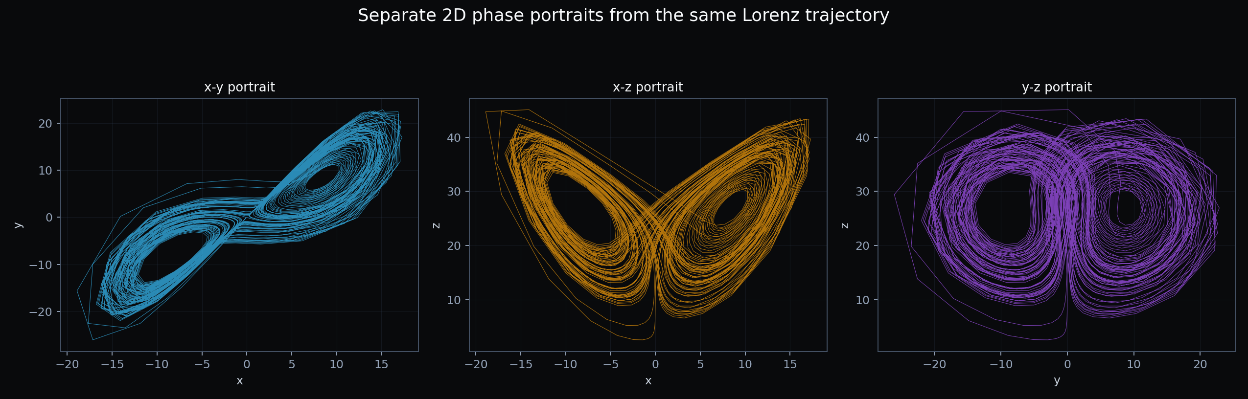
2D Phase Portraits
Select state-variable pairs, reuse a trajectory, and read folds, loops, crossings, and projection artifacts.
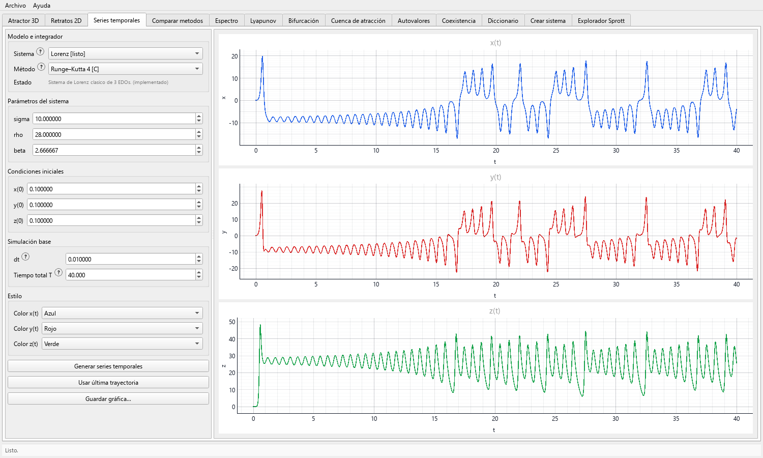
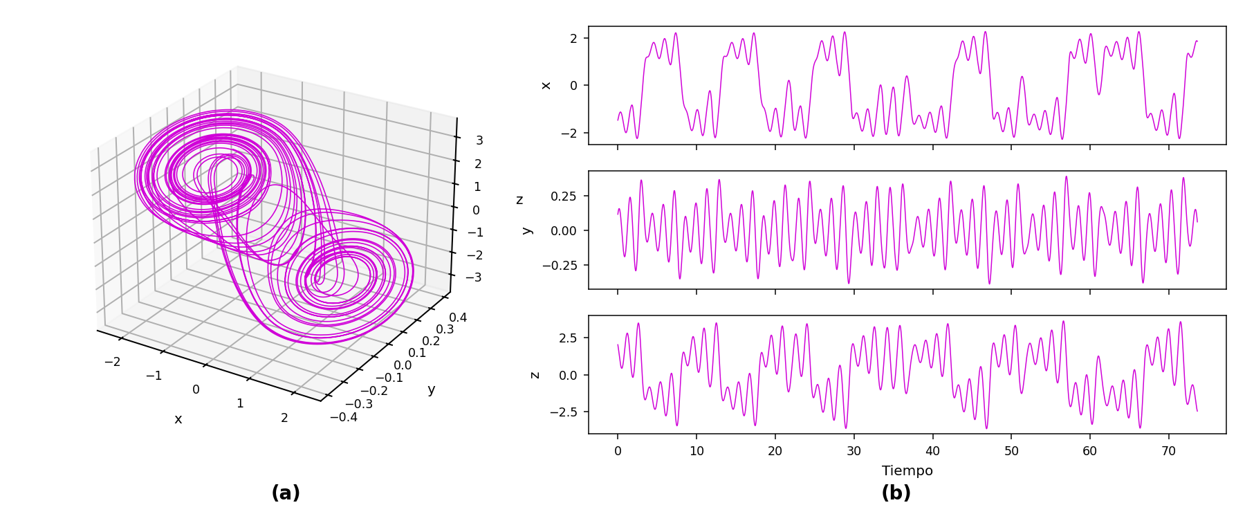
Time Series
Inspect state histories, transients, oscillations, bursts, drift, and numerical failure before deeper analysis.
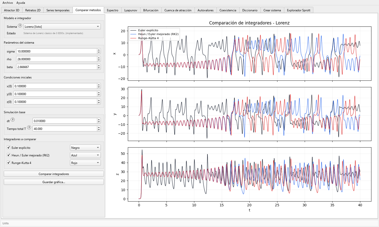
Compare Integration Methods
Compare Euler, Heun, and RK4 under the same numerical contract and perform a practical step-size study.
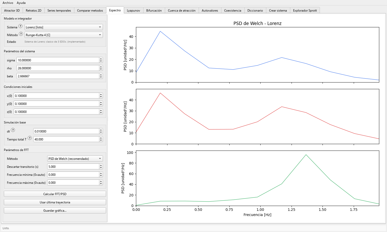
Spectral Analysis
Choose Welch PSD or an amplitude spectrum, discard transients, set frequency limits, and interpret units correctly.
FFT Example
A focused example for generating and reading the Lorenz amplitude spectrum.
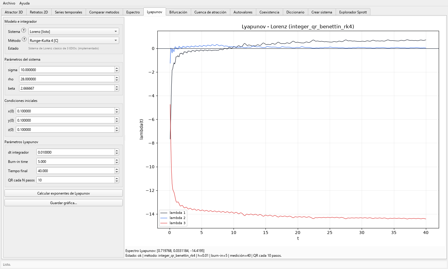
Lyapunov Exponent Diagnostics
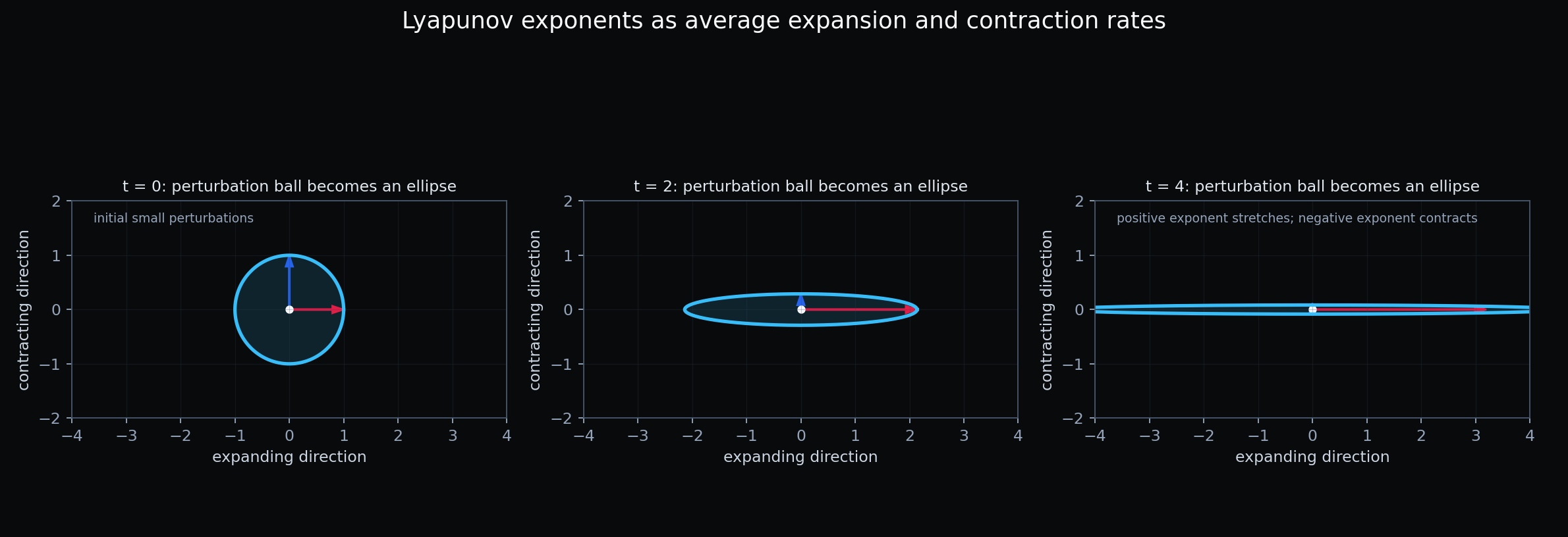
Visualize perturbation growth and read convergence-aware finite-time exponent estimates.
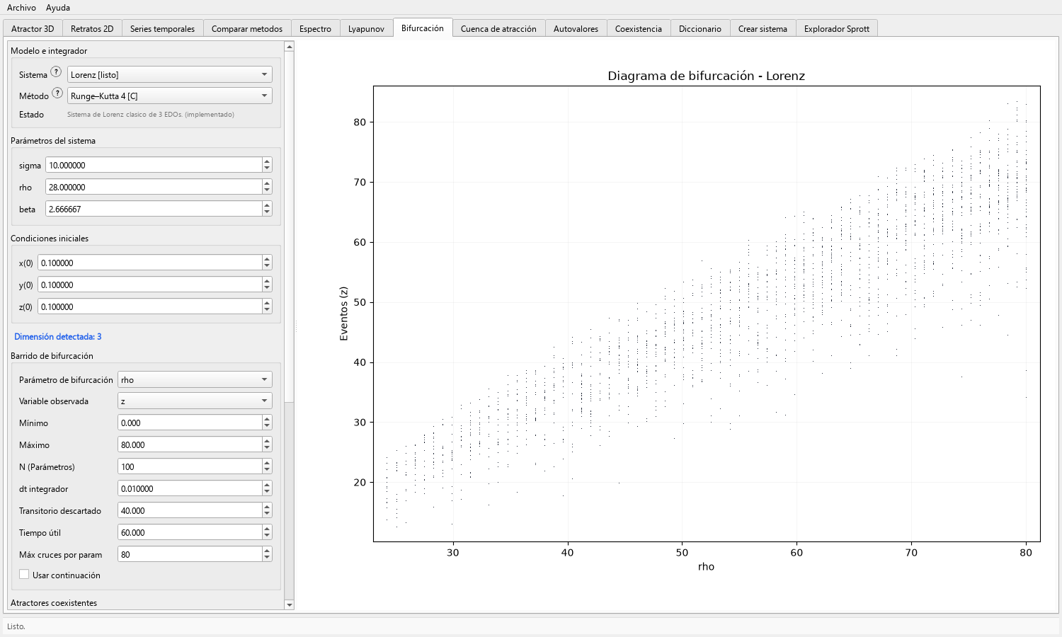
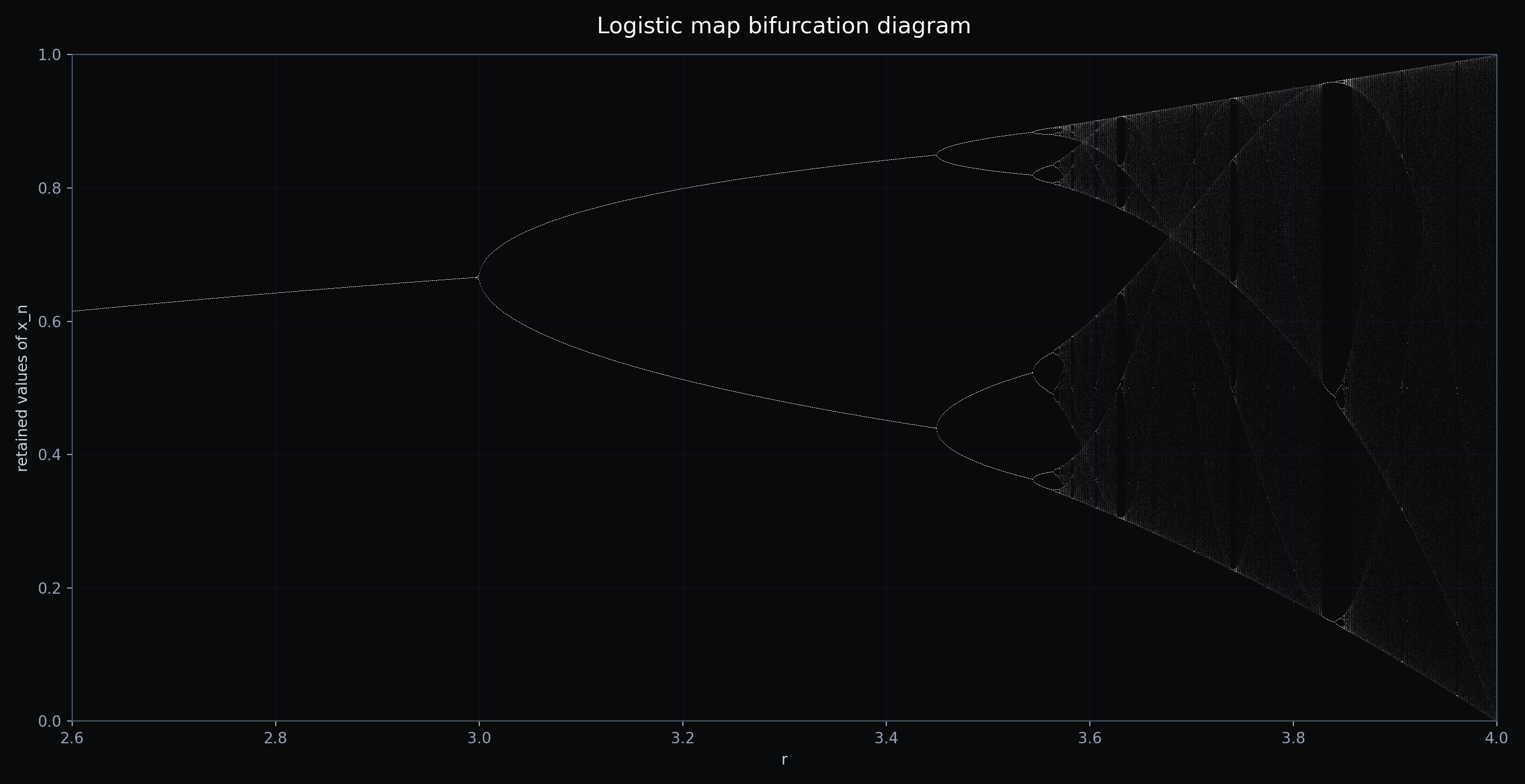
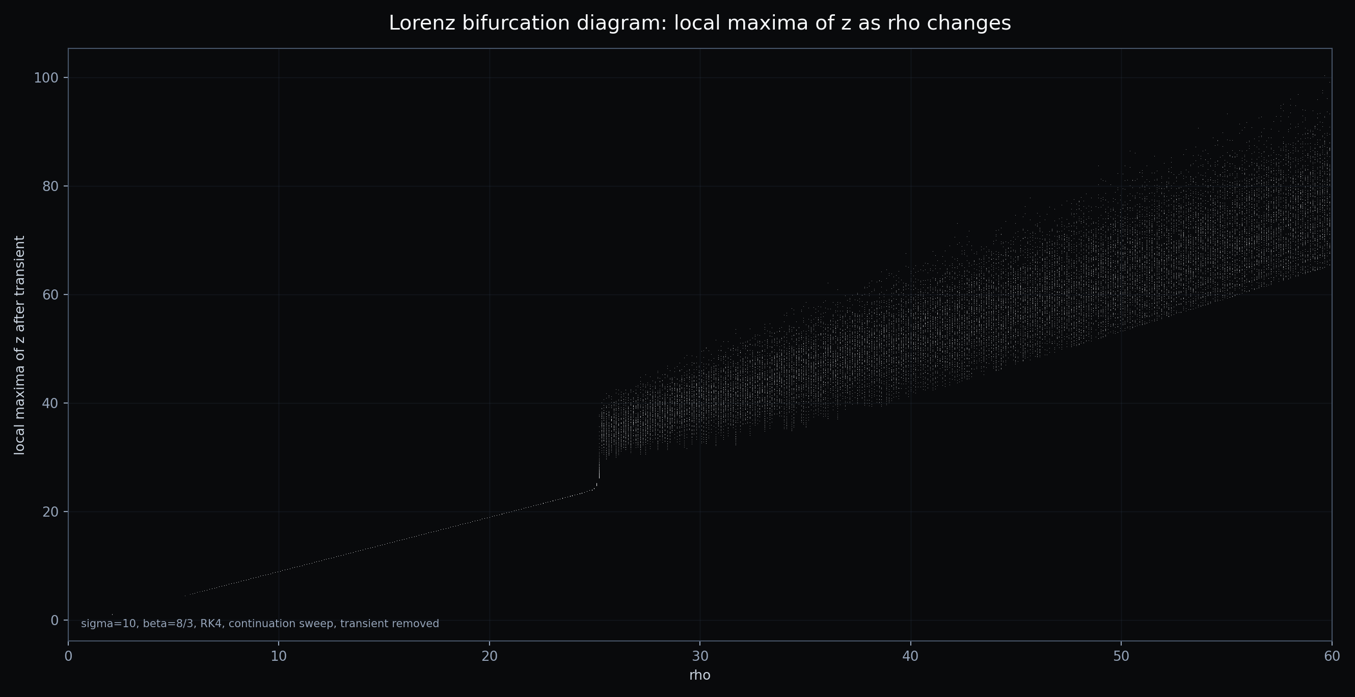
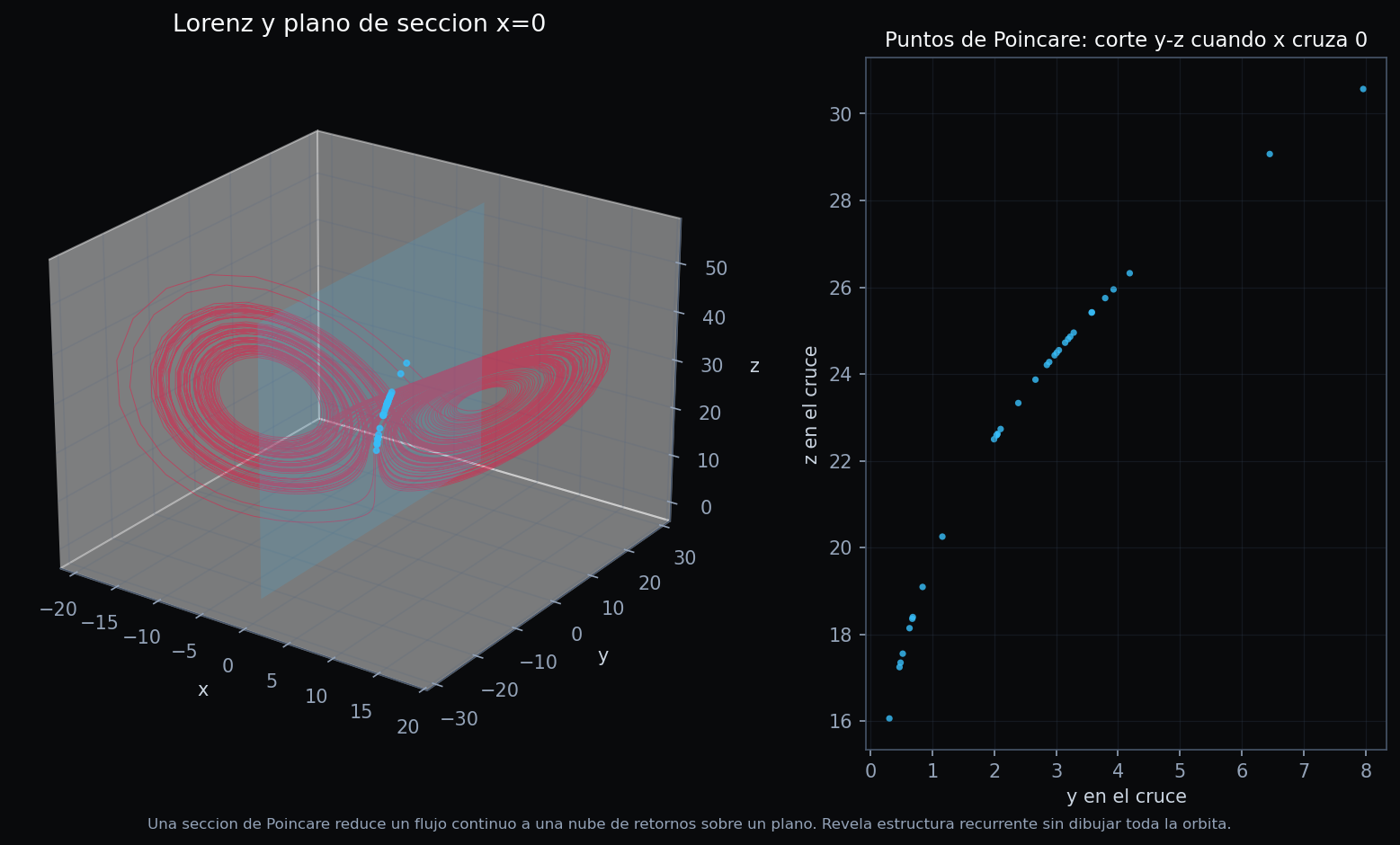
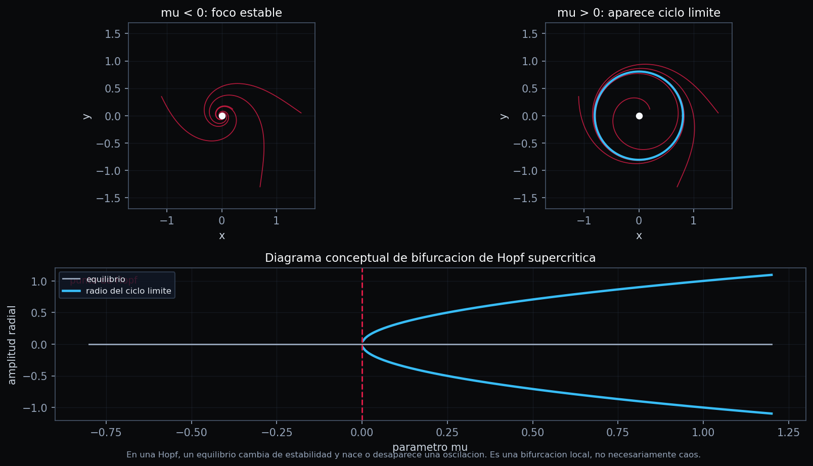
Bifurcation Diagrams
Configure parameter sweeps, retained points, Poincare sections, and Hopf examples.
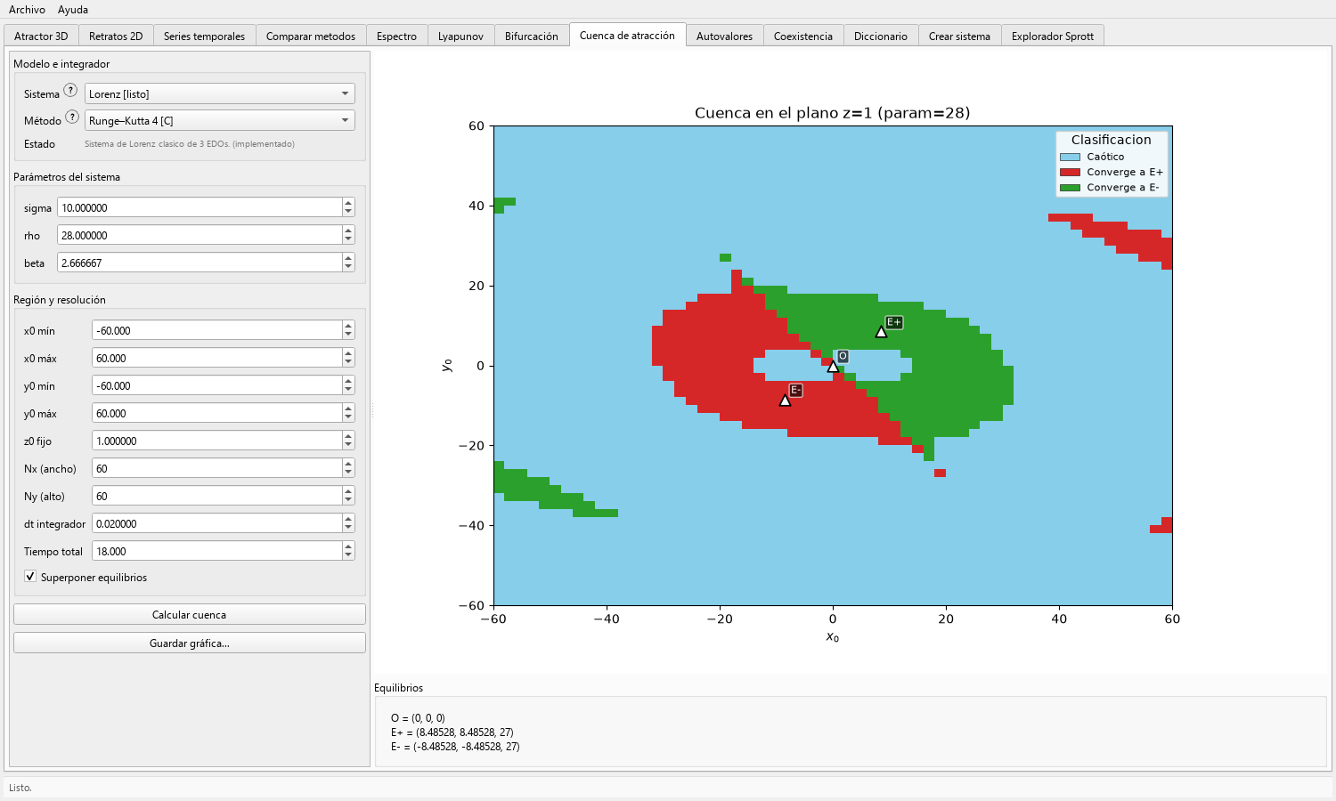
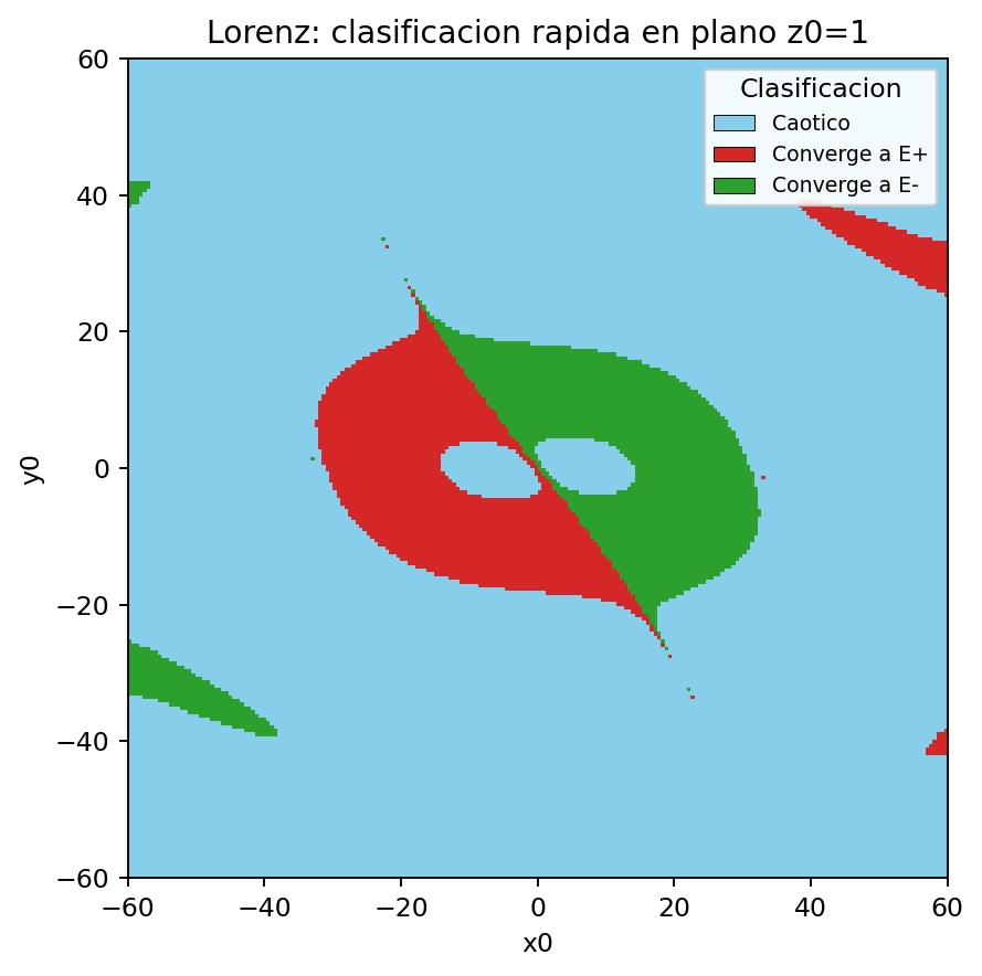
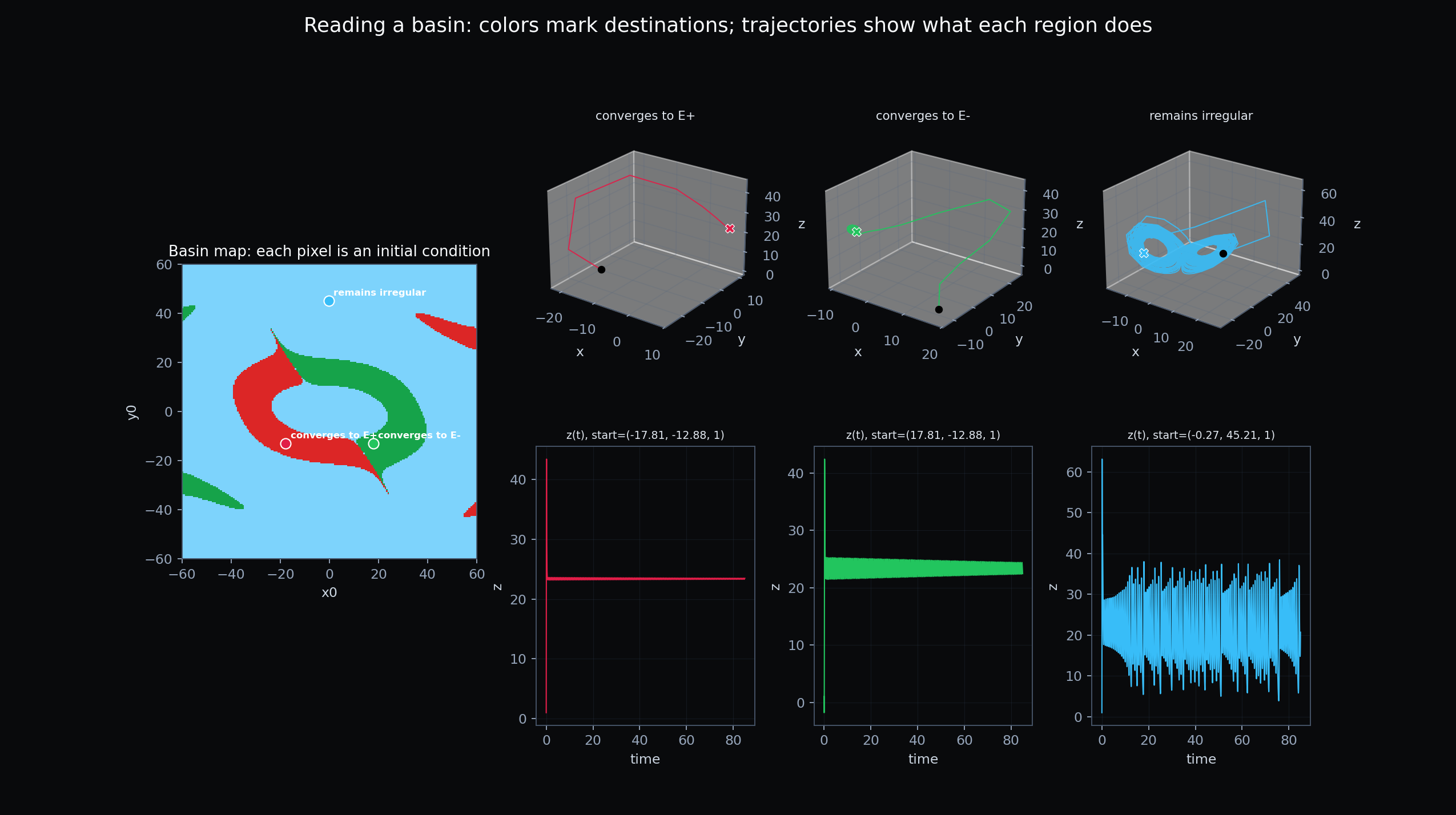
Basins of Attraction
Read finite-resolution basin maps and representative trajectories launched from different regions.
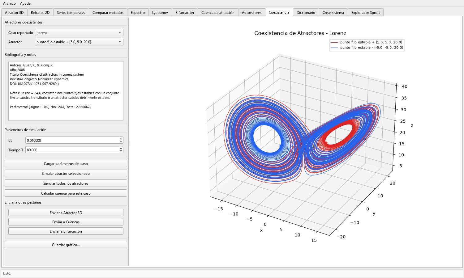
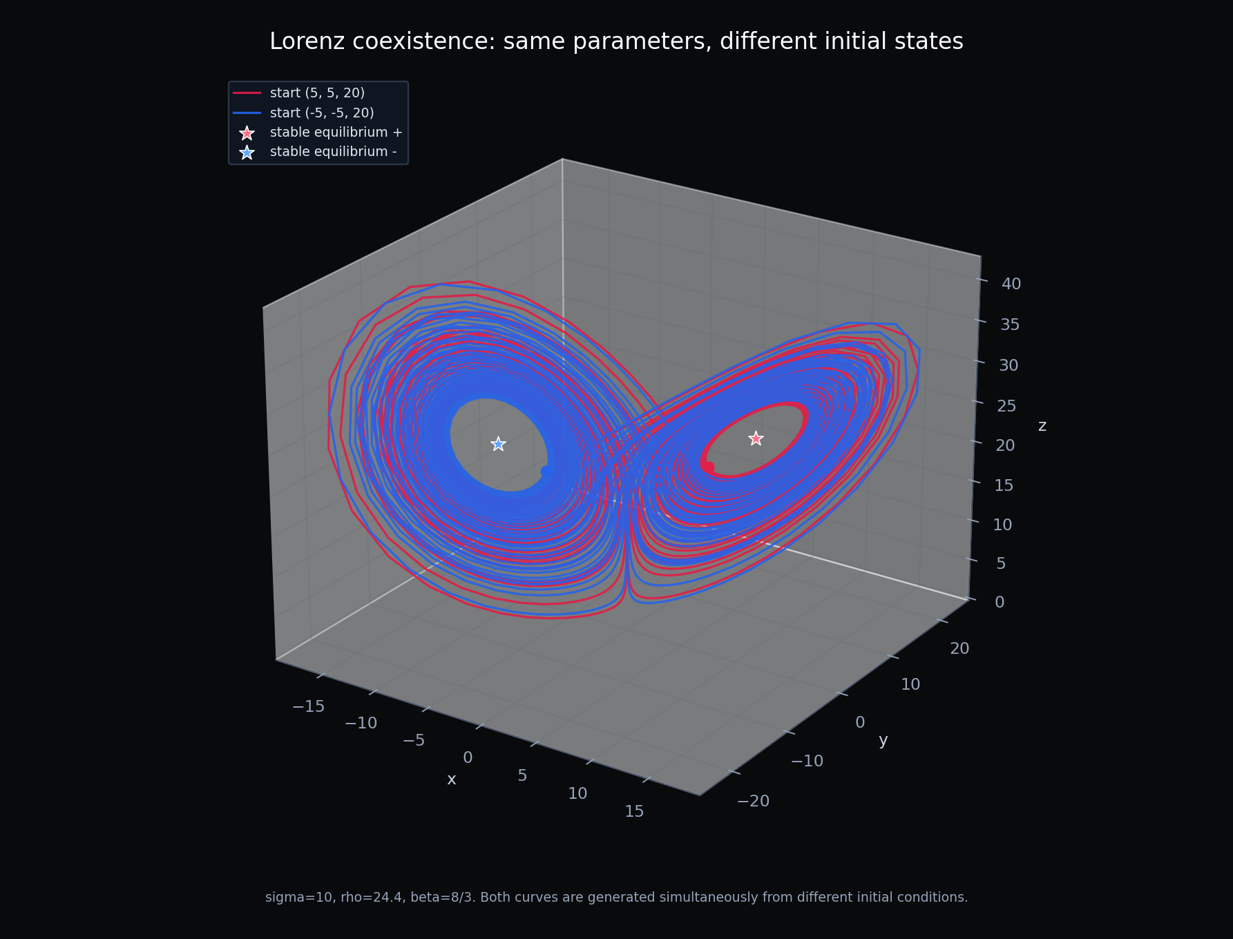
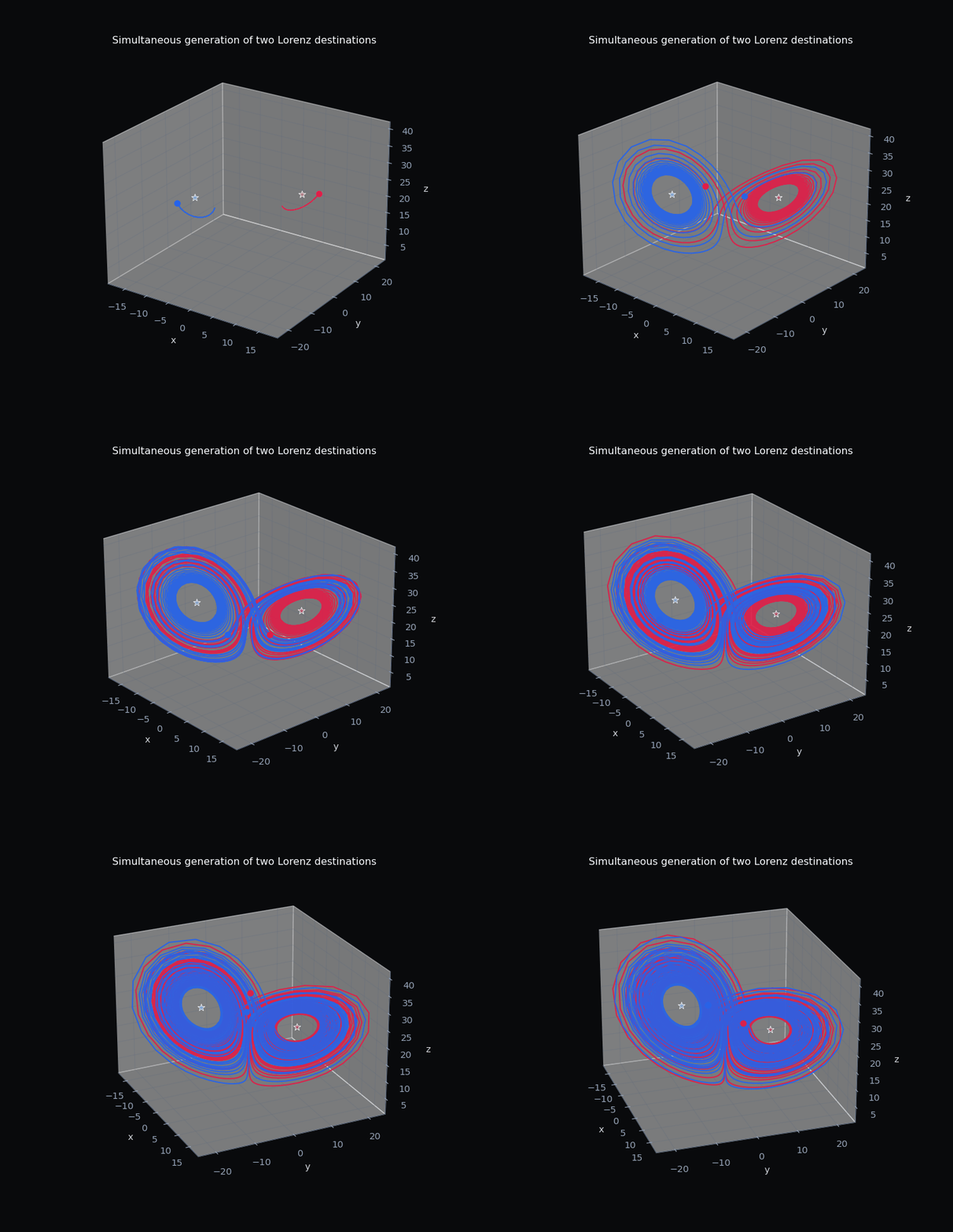
Coexisting Attractors
Compare registered multistability cases under fixed parameters and distinct initial conditions.
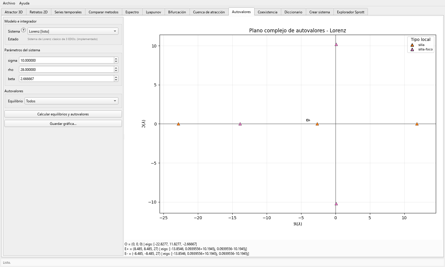
Equilibria and Eigenvalues
Calculate supported ODE equilibria, inspect Jacobian eigenvalues, and report local linear stability responsibly.
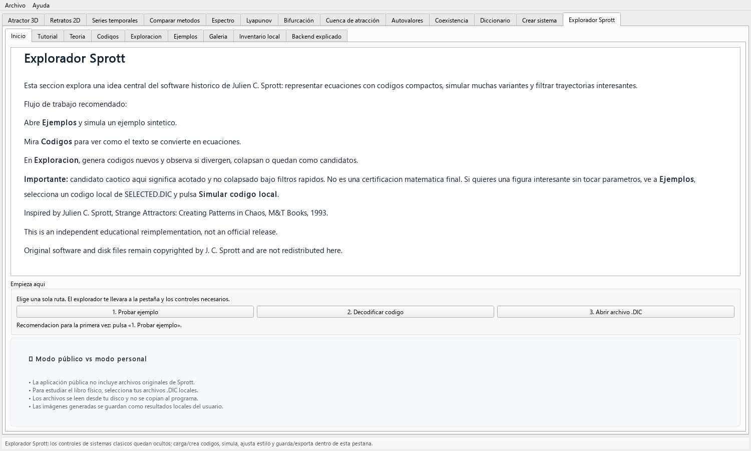
Sprott Explorer
Understand codes, decoding, search, filtering, visual presets, and local user-owned dictionaries.
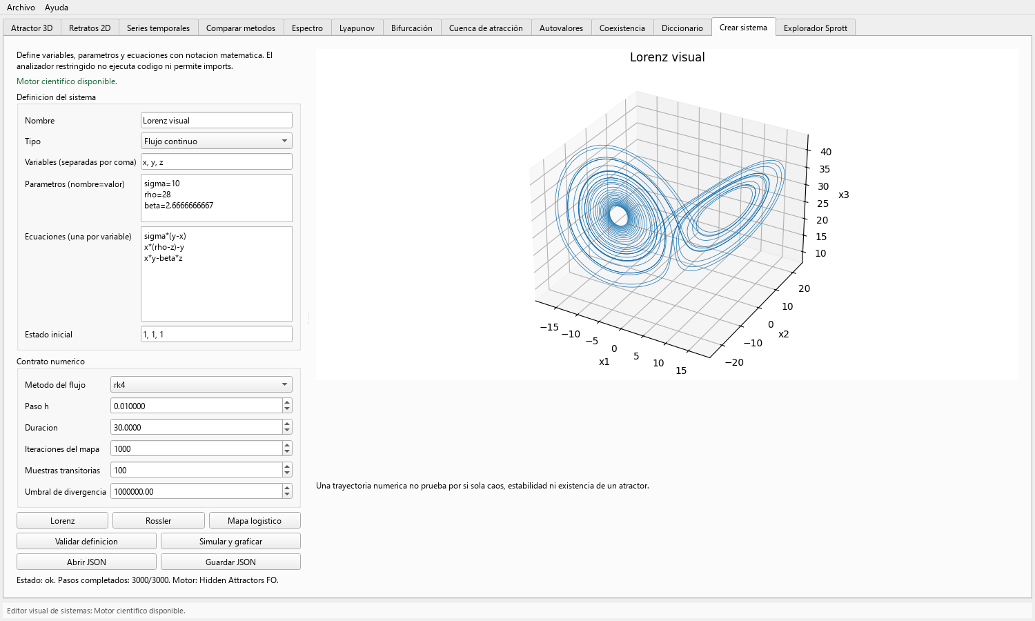
Create a Custom System
Define, validate, simulate, import, and export a flow or map with the no-code editor.
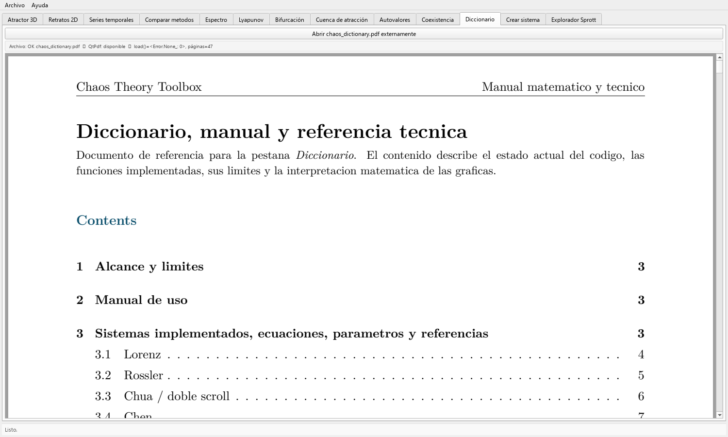
Concept Dictionary
Use the built-in dictionary as a learning aid and connect definitions to plots and numerical experiments.
Export and Reproducibility
Save figures and definitions, record the numerical contract, and build a result package another person can audit.
Research Workflows
Plan parameter studies, comparison matrices, multistability screens, and evidence-preserving exploratory campaigns.
Scientific Interpretation
Separate what plots and finite computations show from claims that require convergence studies or formal analysis.
Visual Output Gallery
Current GUI workspaces plus representative attractors, bifurcations, Poincare sections, basins, coexistence cases, Lyapunov figures, and Sprott-generated graphics.
Citing Fyskode Chaos Toolbox
If you use this software in research, thesis, or academic workflows, cite the archived OSF release.
Maria Fernanda Moreno Lopez. Fyskode Chaotic Systems Toolbox, version 0.1.0. 10.17605/OSF.IO/GQMJR.