Basins of Attraction

Compute and read grid-based basin maps that classify initial conditions by their final destination.

Question Where does each start go?

Use This When You need a grid classification

Objective

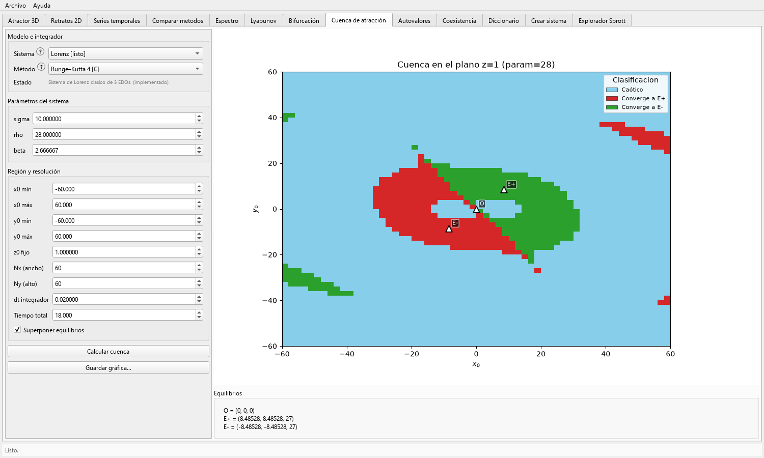
Build a two-dimensional map of initial conditions, compare the computed destination classes, and verify the reading with representative trajectories.

Workspace

GUI tab

Cuenca de atracción

Procedure

Select a supported 3D flow and define its parameters, integration method, step, and total time.
Set the x0 and y0 limits, the fixed z0 coordinate, and a moderate Nx by Ny grid for the first calculation.
Keep Superponer equilibrios enabled when equilibrium markers will help orient the map; the Equilibrios panel reports the coordinates used by the view.
Calculate the basin, inspect escape or unresolved regions, and refine the window, time, or resolution only after the first map is interpretable.
Simulate representative starts from different colors before assigning a dynamical meaning to each class.

Result

Expected result

A color-coded grid in which each sampled initial condition is assigned a computed destination class.
When requested, equilibrium markers over the map and selectable equilibrium coordinates in the adjacent information panel.

Interpretation

The colors are numerical class labels for the selected plane, grid, solver settings, and finite integration time; they are not state-variable values.

Equilibrium overlays provide geometric reference points. They do not replace representative trajectory checks or convergence tests near a boundary.

Export

Export and reproducibility

Use Guardar gráfica to save the basin figure after its legend, limits, and equilibrium markers are readable.
Record the system, ordered parameters, method, dt, total time, x0/y0 window, fixed z0, Nx, Ny, and whether equilibrium overlays were shown.

Applications

Studying sensitivity to initial conditions and multistable destination regions.
Selecting representative starts for later trajectory comparisons and teaching basin concepts.
Comparing how a sampled basin changes under controlled parameter or resolution variations.

Limits

A finite grid can miss small or intricate regions, and a finite horizon can misclassify slow transients.
The displayed slice does not describe the full state space, and an equilibrium marker does not establish attraction from its neighborhood.
This GUI workflow does not locate or certify hidden attractors.

Current Toolbox Chaos Cuenca de atracción tab showing a Lorenz classification — Current interface: each cell is an initial condition on the declared plane, colored by its finite-time destination class.

Lorenz basin map with representative trajectories from different colored regions — Dictionary-style reading: select representative starts from different colored regions, integrate the trajectories, and verify that each color corresponds to a different long-term destination.

What a Basin Means

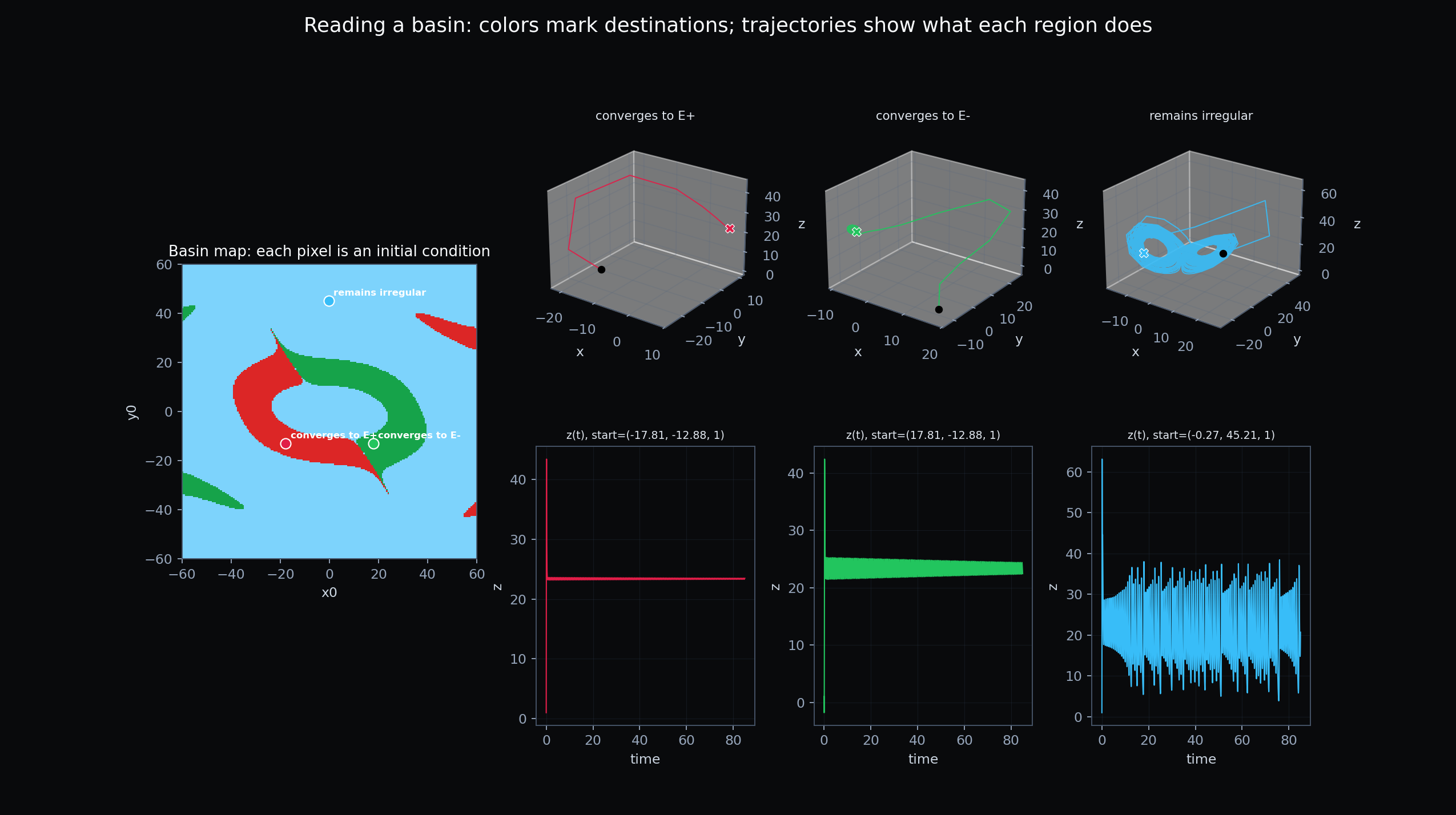
A basin of attraction partitions initial conditions by their final behavior. In a two-dimensional basin plot, the horizontal and vertical axes are two initial coordinates. The third coordinate is held fixed. The solver launches one trajectory from each grid point, integrates it, and classifies the destination after the retained integration window.

The important reading habit is to separate the map from the trajectories. The map tells you which destination belongs to many starts. The representative trajectories show why the colors are meaningful: starts chosen from different regions fall into different final zones.

Steps

Open the attraction-basin workflow in the toolbox.
Select a supported continuous 3D flow such as Lorenz, Chua, or Rossler.
Choose the plane limits with x0 min, x0 max, y0 min, and y0 max.
Set the fixed coordinate, for example z0 = 1 for a Lorenz x-y initial-condition plane.
Use Superponer equilibrios when you want equilibrium markers on the map, and read their coordinates in the Equilibrios panel. Disable the option when the markers would obscure a dense boundary.
Start with a modest grid such as Nx = 120, Ny = 120. Increase resolution only after the region is meaningful.
Run the classification and inspect whether the classes are stable rather than dominated by divergence or unresolved points.
Pick representative initial conditions from different color regions and simulate their trajectories to confirm the basin reading.

How Parameters Change This Figure

Grid resolution: higher Nx and Ny reveal finer basin boundaries but increase computation time.
Integration time: too short can misclassify slow convergence; too long can make high-resolution grids expensive.
Fixed coordinate: changing the fixed coordinate changes the plane being sampled, so the basin shape can change.
Plane window: a wide region gives context; a narrow region is better after you know where the boundary lives.
Classifier thresholds: hit radii, escape radii, and unresolved labels control how final destinations are assigned.

Common Confusion

Basin map: many initial conditions are classified over a grid.
Coexistence plot: a small set of selected trajectories is compared under fixed parameters.
Attractor plot: the long-term geometry of one trajectory is shown in phase space.