Coexisting Attractors

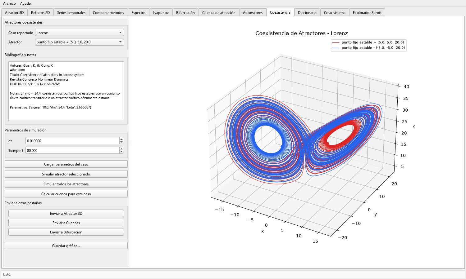
Compare the registered Lorenz coexistence case: same parameters, two initial conditions, and two stable coexisting destinations.

Case Lorenz, rho = 24.4

Use This When Same parameters, different starts

Objective

Compare registered trajectories under one unchanged parameter set and use their different initial conditions to study distinct computed destinations.

Workspace

GUI tab

Coexistencia

Procedure

Select a registered coexistence case and review its reference and parameter set. Coexistence simulations read that registered parameter_set directly; no separate parameter-loading action is required.
Choose one registered attractor or simulate all of them with the same dt and total time.
Confirm that the equations and parameters remain unchanged while only the initial conditions differ.
Use Calcular cuenca para este caso for a direct follow-up: the application switches to Cuenca de atracción, loads the case, and immediately runs the current basin window, grid, step, and total-time configuration.
Use Enviar a Atractor 3D, Enviar a Cuencas, or Enviar a Bifurcación to copy the selected system, parameter values, and selected initial condition into the corresponding workspace.
Review the destination tab's own controls before calculating there; sending a case changes the workspace but does not replace its tab-specific numerical setup.

Result

Expected result

One or more trajectories showing the destinations reached from registered starts under the same model parameters.
A destination workspace preloaded with the selected coexistence case for 3D inspection, basin sampling, or a parameter sweep.
When the direct basin button is used, a newly calculated basin for the loaded case using the Cuenca tab's current sampling controls.

Interpretation

Different computed destinations under identical equations and parameters are finite numerical evidence of coexistence for the tested initial conditions and settings.

The transfer buttons support a consistent follow-up workflow; they do not make a basin map or bifurcation diagram equivalent to the original trajectory comparison.

The direct basin result must be interpreted from its declared plane, grid, and finite integration time, even though it was launched from the coexistence case.

Export

Export and reproducibility

Use Guardar gráfica to save the coexistence view after all trajectories and initial-condition labels are distinguishable.
Record the case, system, ordered parameters, every tested initial condition, method, dt, total time, and any destination-tab settings used after a transfer.

Applications

Teaching multistability and the role of initial conditions under a fixed parameter set.
Selecting cases for 3D views, basin sampling, or bifurcation follow-up without retyping the shared model inputs.
Designing controlled comparisons of candidate destinations and their numerical robustness.

Limits

A comparison of a few registered starts does not map the full basin or establish all possible destinations.
Coexistence does not imply that every displayed destination is chaotic, and finite convergence can be confused with a long transient.
The transfer workflow does not locate or certify hidden attractors.

Current Toolbox Chaos Coexistencia tab showing the registered Lorenz case — Current interface: the registered Lorenz case keeps one parameter set and compares the trajectories from both documented initial conditions.

Animation of two Lorenz coexisting trajectories generated at the same time — Simultaneous-generation animation: both trajectories use the same equations and parameters. Only the initial condition changes.

Theory

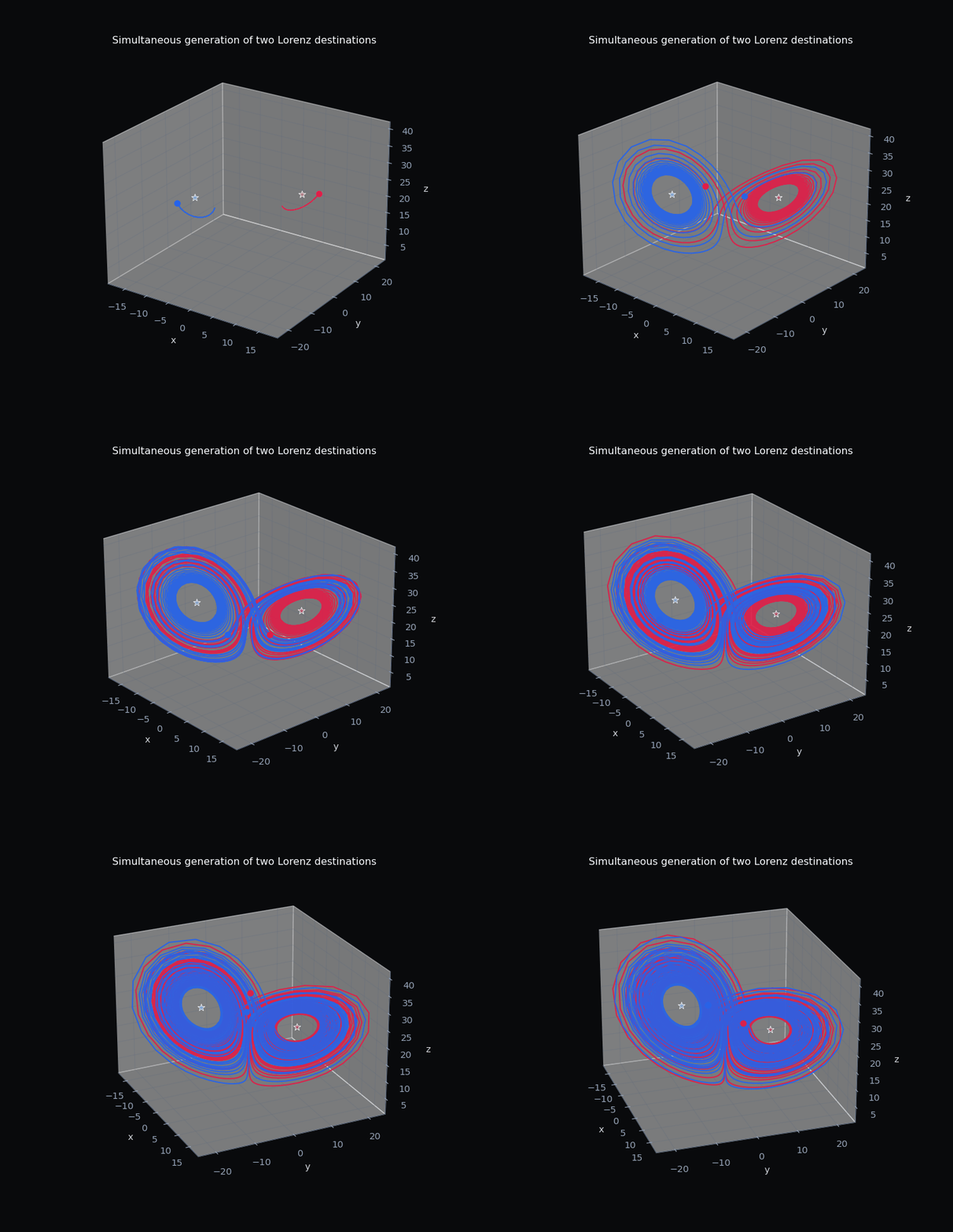
Coexistence means that the equations and parameters stay fixed, but changing only the initial condition can lead to a different long-term behavior. In the Lorenz case used by the toolbox, the parameter set is not the classical chaotic one with rho=28. It uses sigma=10, rho=24.4 and beta=8/3, where the registered starts approach two different stable equilibria.

This is a central idea for multistability. The system is not described only by its equations; it is also shaped by the region of phase space where the experiment begins. For students, the important lesson is that one simulation is not enough to describe a multistable system.

Steps

Open the coexistence workflow in the toolbox.
Select the registered Lorenz coexistence case.
Review the registered values sigma = 10, rho = 24.4, and beta = 8/3. The simulation actions read this case parameter set automatically.
Compare the registered initial conditions (5,5,20) and (-5,-5,20).
Simulate both trajectories in the same figure.
Read the final destinations: one trajectory approaches the positive stable fixed point and the other approaches the negative stable fixed point.
For an immediate grid study, first review the window, fixed coordinate, resolution, dt, and total time in Cuenca de atracción. Return to Coexistencia and press Calcular cuenca para este caso; the application loads the case in that tab and starts the basin calculation directly.
Select one registered attractor and use Enviar a Atractor 3D, Enviar a Cuencas, or Enviar a Bifurcación to copy its system, parameters, and initial condition. Review the receiving tab's controls, then run the requested analysis there.

How Parameters Change This Figure

Initial condition: this is the main control in coexistence. Changing only the start can change the destination.
rho: rho=24.4 shows two stable Lorenz equilibria; rho=28 shows the classical chaotic Lorenz attractor and is a different lesson.
Total time: too short can show only transients. The destination is read after the trajectory has settled.
Step size: too large a step can move a trajectory into the wrong destination numerically.
View angle: rotation changes how clearly the symmetric destinations separate in the 3D figure.

Common Confusion

Coexistence is not a basin: a coexistence plot compares selected trajectories; a basin map classifies many initial conditions on a grid.
Coexistence does not always mean two chaotic attractors: the Lorenz example here shows two stable fixed points for the same parameter set.
Same parameters matter: if you change parameters between runs, you are no longer testing coexistence.