Toolbox Chaos practical guide
Getting Started with Toolbox Chaos
Go from the desktop installer to a first catalog simulation, reuse the same trajectory in another view, and save a research-ready figure.
Objective
What you will accomplish
Complete one traceable simulation without writing code and learn the small set of controls that appears throughout the interface.
Before you begin
- Install the build for your operating system and open Toolbox Chaos from the normal application shortcut.
- Choose a folder where you can keep figures and a short text record of the parameters used.
- No Python environment or command line is required for this GUI workflow.
Reference outputs
What these views can show
Procedure
Step-by-step workflow
-
Open the first simulation panel
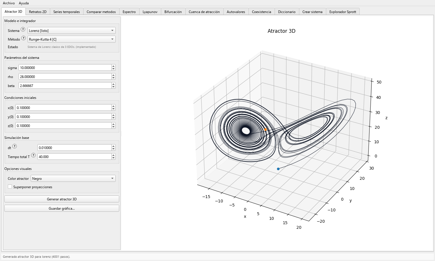
Select Atractor 3D. The left panel contains the system, parameter, initial-condition, method, step-size, and duration controls; the right panel is the plot area.
If your display is narrow, scroll the control panel rather than reducing the application window until buttons disappear.
-
Load a catalog model
Choose Lorenz. The catalog fills its documented parameter order, initial state, and numerical defaults automatically.
For the first run, retain sigma = 10, rho = 28, beta = 8/3 and a small nonzero initial state. Record any value you change.
-
Declare the numerical contract
Select Runge-Kutta 4, use a step near 0.01, and use a duration long enough to pass the initial transient.
The method, step, duration, initial state, and parameters jointly define the experiment; the system name alone is not enough to reproduce it.
-
Generate and inspect
Press Generar atractor 3D and wait for the status message to confirm completion.
Rotate the view, check that the trajectory remains finite, and look for both Lorenz lobes. A blank, exploding, or needle-like result is a reason to review the contract before continuing.
-
Reuse the trajectory
Open Retratos 2D or Series temporales, keep the same system selected, and press Usar última trayectoria.
This avoids accidentally comparing different integrations while learning how geometric and temporal views complement one another.
-
Save the result
Use Guardar gráfica and choose PNG for slides or web use, PDF for scalable document insertion, or another offered raster format.
Store a companion note with the system, complete parameter vector, initial condition, method, step, duration, application version, and which transient portion you interpreted.
Result
Expected output
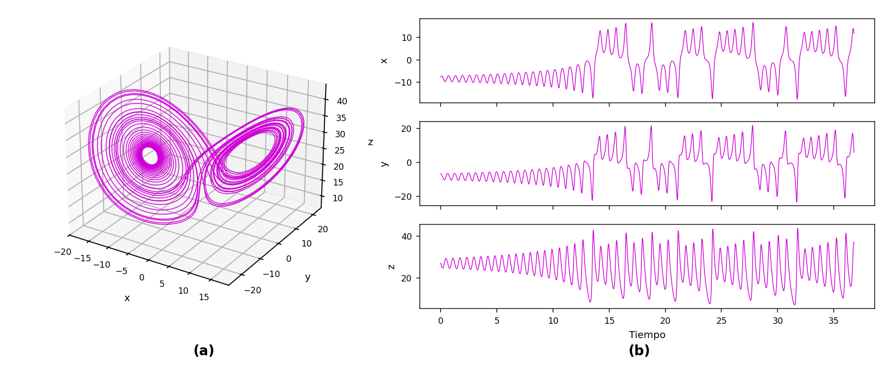
- A bounded Lorenz trajectory with two lobes in 3D and matching state traces or pairwise projections when the shared trajectory is reused.
- At least one saved image plus enough numerical metadata to repeat the run.
- A clear distinction between selecting a named example and making a scientific classification about its behavior.
Interpretation
How to read it
The 3D curve is the computed history of the state vector, not a path through ordinary physical space. The two lobes describe regions repeatedly visited by this finite trajectory.
Irregular lobe switching is compatible with the familiar Lorenz chaotic regime, but the plot by itself is not a proof. Confirm conclusions with time series, step refinement, longer horizons, and a suitable diagnostic.
Export
Reproducibility checklist
- Save the figure with a descriptive name such as lorenz_rho28_rk4_h001.
- Record parameter order as displayed by the GUI; do not rely on memory or alphabetical order.
- Record whether the output is a fresh local simulation or a reused shared trajectory.
- Keep the raw experiment notes with the final figure so later styling does not erase provenance.
Applications
Where this workflow helps
- First laboratory exercise on phase space and sensitivity to initial conditions.
- Baseline run before a parameter sweep, method comparison, spectrum, or Lyapunov calculation.
- Rapid visual screening of a catalog system before designing a reproducible research protocol.
Limits
What it does not establish
- The 3D tab is intended for three-state views; use 2D portraits or time series when the selected model has another displayed dimension.
- A single trajectory cannot establish attraction, asymptotic chaos, multistability, or robustness.
- Toolbox Chaos does not locate or certify hidden attractors. That scientific task is outside this GUI workflow.