Toolbox Chaos practical guide
Research Workflows
Turn GUI exploration into bounded, traceable studies of parameters, initial conditions, numerical sensitivity, spectra, stability, and multistability.
Objective
What you will accomplish
Design an exploratory campaign in which every claim has a matching GUI operation, saved output, and verification step.
Before you begin
- Write a specific question, independent variables, fixed controls, output metrics, and stopping criterion before running a large grid.
- Establish a baseline simulation and a reproducible export convention.
- Distinguish exploratory evidence from formal proof and from specialized analyses performed outside Toolbox Chaos.
Reference outputs
What these views can show
Procedure
Step-by-step workflow
-
Frame one testable question
Examples include how a portrait changes with one parameter, whether a spectral peak persists under refinement, or whether registered initial conditions reach visibly distinct long-time states.
Avoid broad goals such as ‘find chaos.’ Define the computed output and what outcome would be considered continue, reformulate, or discard.
-
Establish the baseline
Use Atractor 3D, Retratos 2D, and Series temporales to check boundedness, transient duration, state scale, and useful observables.
Use Comparar métodos and step refinement before committing to a costly sweep.
-
Choose the exploration axis
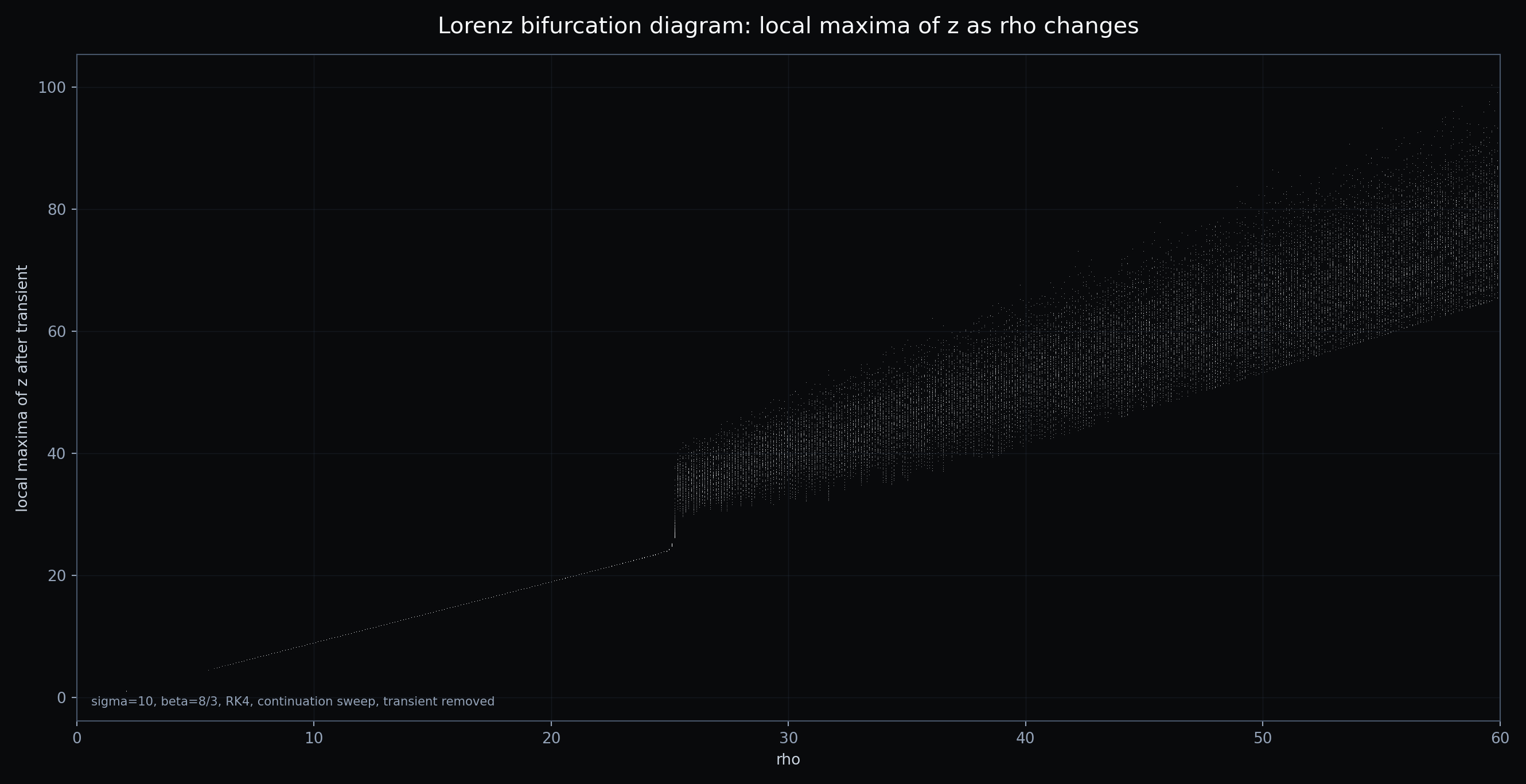
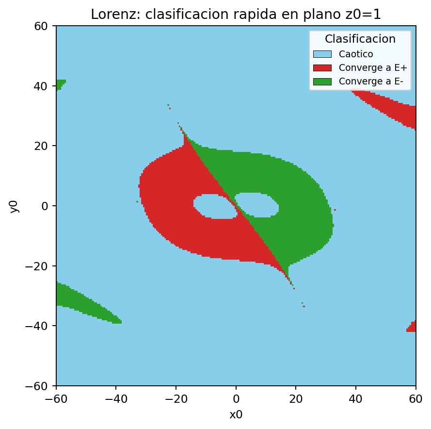
For one model parameter, use Bifurcación with a declared range and sampling density. For initial states, use Coexistencia or Cuenca de atracción only where their registered cases or classifiers are supported.
For a small hypothesis-driven comparison, use a run matrix with one changed factor and saved portraits, time series, or spectra.
-
Add the matching diagnostic
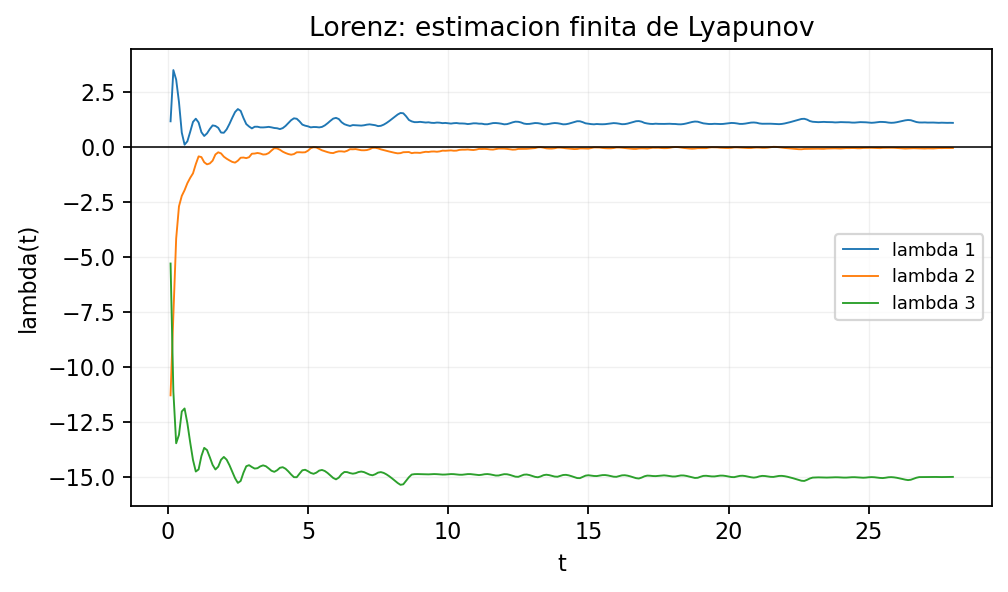
Use Espectro for frequency structure, Lyapunov for the supported finite-time 3D ODE-flow calculation, and Autovalores for supported local equilibrium analysis.
No diagnostic should be used outside the model type, dimension, or numerical contract stated by its tab.
-
Repeat and refine
Repeat selected cases with a smaller step, longer horizon, different transient, and nearby initial states. Increase sweep or basin resolution only after the coarse campaign identifies a bounded region worth refining.
Preserve divergent, inconclusive, and contradictory cases; they determine the limits of the study.
-
Report an evidence matrix
For each conclusion, list the direct output, numerical checks, alternative explanations, and remaining limitations.
Use language such as ‘finite-time estimate,’ ‘at the tested grid resolution,’ and ‘for the sampled initial conditions’ whenever those qualifiers define the evidence.
Four reusable study patterns
- Parameter study: baseline → bifurcation sweep → selected portraits/time series → diagnostic → step and grid refinement.
- Initial-condition study: fixed parameters → declared plane/domain → basin or registered coexistence comparison → representative trajectories → resolution and horizon checks.
- Numerical study: fixed model → Euler/Heun/RK4 comparison → step ladder → stable summary quantities → method choice with limitations.
- Custom-model pilot: validate JSON definition → baseline simulation → independent equation check → numerical refinement → decide whether specialized code is needed.
Result
Expected output
- A baseline plus a structured parameter or initial-condition campaign with declared controls.
- A set of figures and settings records linked to specific research questions.
- An evidence matrix that distinguishes supported conclusions, provisional inferences, and unresolved cases.
Interpretation
How to read it
A robust exploratory finding persists across relevant resolution and horizon changes and appears in more than one appropriate view or diagnostic.
Contradictory diagnostics are not a reason to select the preferred plot; they indicate a transient, numerical, model-compatibility, or interpretation question that must be resolved.
Export
Reproducibility checklist
- Predeclared question, varied factor, fixed controls, grid, and stopping rule.
- Baseline and refinement runs with complete numerical contracts.
- All direct outputs, including failures and null or unresolved cases.
- A claim-to-evidence table and a separate list of analyses performed outside the GUI.
Applications
Where this workflow helps
- Parameter-regime mapping and hypothesis generation.
- Numerical-method sensitivity studies.
- Teaching laboratories on bifurcation, spectra, stability, and multistability.
- Preparation of bounded pilot studies before custom code or high-performance campaigns.
Limits
What it does not establish
- Toolbox Chaos is an exploratory GUI; large campaigns may require scripted workflows, external statistics, or specialized solvers.
- Finite parameter and initial-condition grids cannot establish global completeness.
- Hidden-attractor localization and certification are exclusively part of the separate Hidden Attractors FO research workflow, not a Toolbox Chaos research claim.