Toolbox Chaos practical guide
Equilibria and Eigenvalues
Compute supported ODE equilibria, inspect their Jacobian eigenvalues in the complex plane, and distinguish local linear stability from global dynamics.
Objective
What you will accomplish
Use equilibrium and eigenvalue information as a local analysis layer that complements, but does not replace, trajectories and parameter studies.
Before you begin
- Select a supported continuous ODE flow; maps, delay models, and special high-dimensional cases may not be available in this panel.
- Understand that eigenvalues describe the Jacobian linearization at a particular equilibrium and parameter set.
Reference outputs
What these views can show
Procedure
Step-by-step workflow
-
Select the ODE and parameters
Choose the system and enter its parameter values. Initial condition, integration method, and duration are intentionally absent because the equilibrium calculation is not a trajectory integration.
Record the parameter vector before calculating; changing a parameter can move, create, merge, or remove equilibria.
-
Calculate the supported equilibria
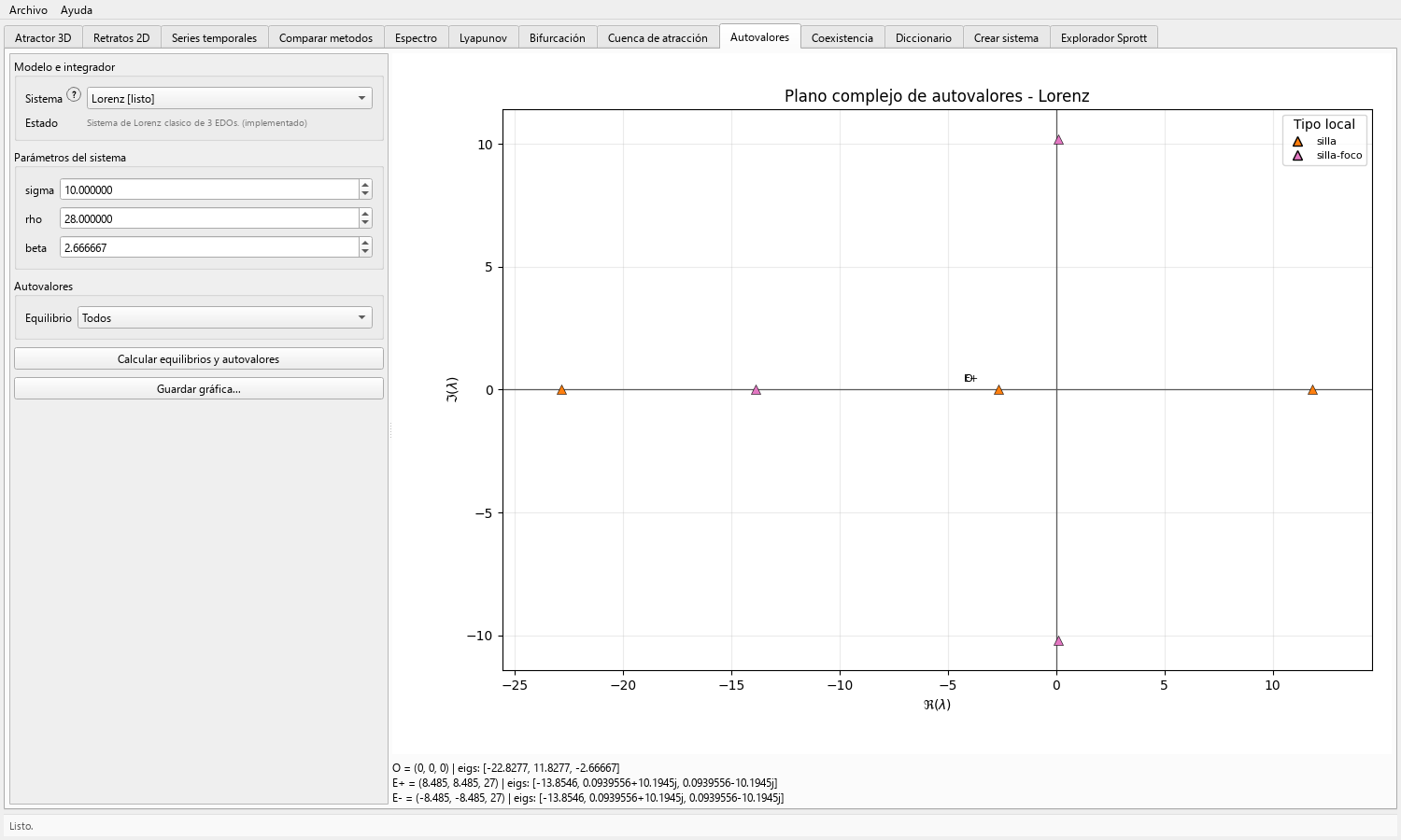
Press Calcular equilibrios y autovalores. The panel displays the supported equilibrium set and corresponding eigenvalues in its information area and complex-plane figure.
If the interface reports that the calculation is unavailable, do not infer that the system has no equilibria; it means the panel lacks that supported contract for the selected model type.
-
Inspect all points
Choose Todos to plot all returned eigenvalues in the complex plane and read the coordinate list in the information area.
Check multiplicity, complex-conjugate pairs, and real parts near zero, which can make finite-precision classification delicate.
-
Inspect one equilibrium
Select an individual equilibrium to view its point, eigenvalues, local type, and classification.
Relate signs of real parts to local contraction or expansion only within the assumptions of linearization; nonhyperbolic cases require additional analysis.
-
Connect local and global views
Run trajectories from small, explicitly declared perturbations only when the research question requires local numerical behavior.
Use phase portraits, time series, and parameter sweeps to study global behavior; eigenvalues do not describe an entire basin or distant invariant set.
-
Preserve the figure and displayed values
Save the complex-plane figure and record the equilibrium coordinates and eigenvalue values exactly as shown in the information area.
The information area rounds equilibrium coordinates with .4g formatting and eigenvalues with .6g formatting. The tab does not offer a full-precision data or table export, so retain the parameter vector and figure with the record.
State whether the view contains all displayed equilibria or one selected point.
Reporting language
- Supported: ‘At these parameters, the panel returned equilibrium E and the Jacobian eigenvalues had these real parts.’
- Supported: ‘At the values displayed by the GUI, the panel labeled this equilibrium with the reported local classification.’
- Not supported by this panel alone: ‘The global dynamics are chaotic,’ ‘the attractor is unique,’ or ‘a hidden attractor has been located.’
Result
Expected output
- Displayed equilibrium coordinates and Jacobian eigenvalues for one parameter vector, formatted at the precision shown by the interface.
- A complex-plane plot and a cautious local classification for each selected equilibrium.
Interpretation
How to read it
Negative real parts support local linear contraction for a hyperbolic equilibrium; positive real parts indicate expanding directions. Mixed signs indicate saddle behavior, and imaginary parts describe local oscillatory components.
Zero or nearly zero real parts, equilibrium manifolds, and nonlinear degeneracies require analysis beyond a simple eigenvalue sign rule.
Export
Reproducibility checklist
- Record equations or catalog name and the complete parameter vector before calculating.
- Retain the saved complex-plane figure and the equilibrium coordinates, eigenvalues, and local classification exactly as displayed.
- Do not describe the display-formatted coordinates or eigenvalues as full-precision data or promise a table export that the tab does not provide.
- State local classification and avoid global language unless supported by separate evidence.
Applications
Where this workflow helps
- Teaching linearization and local stability.
- Choosing parameter regions for bifurcation exploration.
- Relating local saddle directions to observed trajectory geometry as a hypothesis for further study.
Limits
What it does not establish
- The panel is limited to supported ODE-flow equilibrium contracts.
- Local eigenvalues do not determine global basin geometry, multistability, or the existence of a distant attractor.
- Equilibrium analysis in Toolbox Chaos must not be presented as hidden-attractor localization or certification.