Bifurcation Diagrams

Configure parameter sweeps, retained points, Poincare sections, and Hopf examples to visualize qualitative changes in dynamics.

Difficulty Level Beginner

Question What changes with a parameter?

Objective

Sweep one model parameter, retain a controlled long-term observable, and identify parameter intervals that deserve a more focused simulation.

Workspace

GUI tab

Bifurcación

Procedure

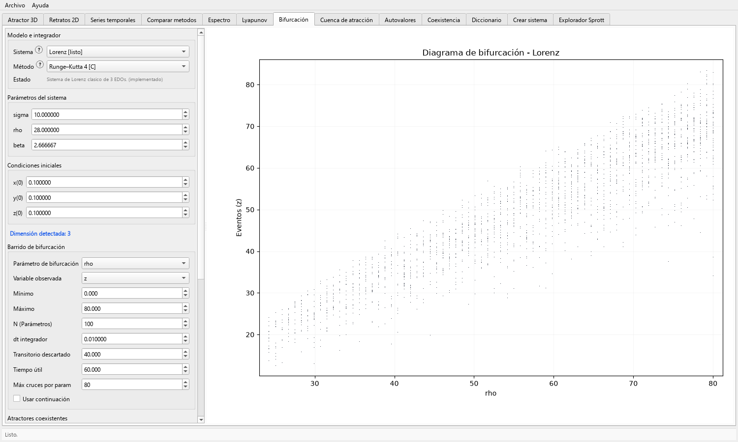
Select the system, the parameter to sweep, and the observed variable, then define the minimum, maximum, and number of parameter samples.
Set the integration step, discarded transient, useful time, and maximum crossings or retained values per parameter.
Enable Usar continuación when each parameter value should start from the final state obtained at the preceding value; leave it disabled to restart from the declared initial condition at every value.
Enable Comparar atractores coexistentes to run the same sweep from initial conditions A and B; select both registered cases or edit their coordinates, then assign contrasting colors.
Calculate the diagram, repeat with a denser local range when needed, and compare continuation on and off whenever path dependence may affect the branches.
Export only after the parameter range, sampling density, and plotted observable are recorded.

Result

Expected result

A parameter-versus-observable point cloud showing retained branches, crossings, or dense response bands.
With continuation enabled, a sweep that follows the numerically reached state from one parameter value to the next.
In A/B mode, two labeled datasets overlaid with the same sweep controls so their initial-condition dependence can be compared.

Interpretation

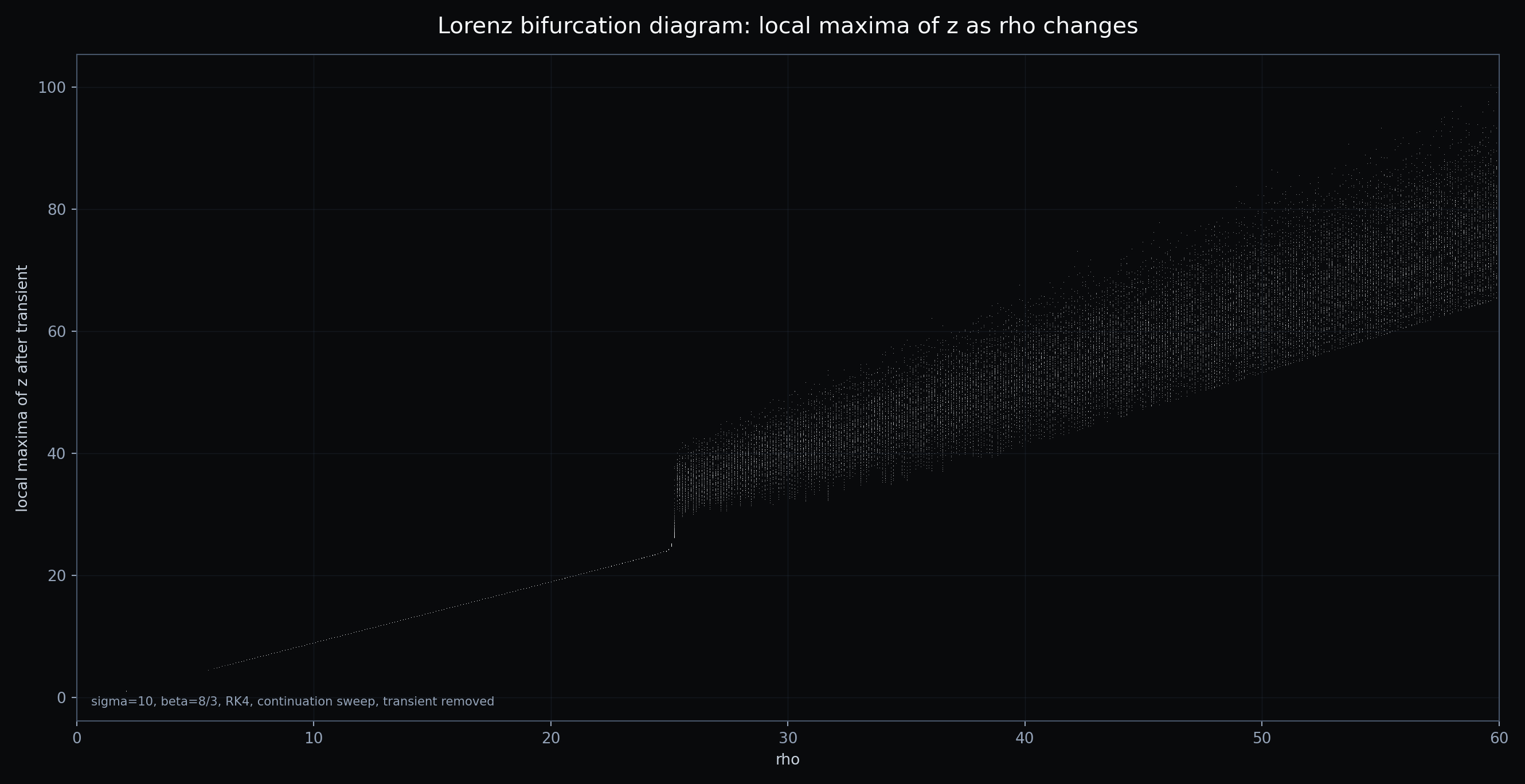
Branch splitting and dense bands identify qualitative changes worth examining, but their appearance depends on the observable, transient, sampling rule, sweep direction, and numerical settings.

A difference between continuation and independent restarts is evidence of path or initial-state dependence in the finite sweep, not by itself a global bifurcation classification.

Separation between the A and B datasets applies only to the two declared starts and the tested parameter path; overlap does not rule out other coexisting responses.

Export

Export and reproducibility

Use Guardar gráfica after axis labels and dense regions remain legible at the intended publication size.
Record the system, ordered parameters, swept parameter and range, observed variable, N, method, dt, transient, useful time, maximum points, continuation state, and—when used—the A/B initial conditions, labels, and colors.

Applications

Locating parameter windows for follow-up trajectories, spectra, or Lyapunov diagnostics.
Teaching fixed branches, period changes, return structures, and the effect of sweep design.
Comparing numerical methods or experimental parameter ranges under a common measurement rule.

Limits

A bifurcation-looking branch can be altered by insufficient transient removal, coarse sampling, a large integration step, or the selected observable.
Continuation can follow one reachable branch while missing alternatives; an independent restart can also miss states outside its chosen initial condition.
The A/B comparison samples two declared starts and is not an exhaustive search for every coexisting response.
The diagram does not prove chaos, attraction, uniqueness, or hiddenness.

Current Toolbox Chaos Bifurcación tab showing a Lorenz rho sweep — Current interface: a moderate-density Lorenz rho sweep retains Poincare events after the declared transient.

High-density Lorenz bifurcation diagram over rho — Flow reference: a larger, higher-density Lorenz rho sweep plots retained local maxima of z so the branches and dense regions are readable.

Lorenz Poincare section showing returns on a plane — Poincare section: a continuous Lorenz trajectory is reduced to return points on a selected plane. This helps compare recurrent structure without plotting every time step.

Conceptual Hopf bifurcation example — Hopf example: an equilibrium changes stability and a small oscillation appears. This explains local onset of oscillations, not an automatic transition to chaos.

Steps

Open the bifurcation workflow in the toolbox.
Select the system to sweep. Start with Logistic for a fast map example or Lorenz for a flow example.
Choose the control parameter, for example r for Logistic or rho for Lorenz.
Set a coarse interval first, such as r = 2.8 to 4.0 for Logistic or rho = 0 to 60 for Lorenz.
Remove enough transient behavior so the plot shows retained long-term values rather than startup motion.
Choose how the sweep is initialized: with Usar continuación enabled, the final state at one parameter value becomes the start for the next; disabled, every value restarts from the declared initial condition. Compare both settings when branch selection matters.
For a controlled two-start comparison, enable Comparar atractores coexistentes, choose Atractor A and Atractor B, verify both initial-condition triples, and select contrasting colors. The tab applies the same parameter sweep and numerical settings to both datasets.
Increase the number of parameter samples and retained points only after the interval is meaningful.
Export a large figure when branches and dense regions are legible.

Theory

A bifurcation diagram is a compact visual summary of how a dynamical system changes when one parameter varies. For each parameter value, the simulation discards the transient and plots retained long-term values. A single branch suggests a stable fixed behavior; two, four, or many branches suggest periodic structure; dense bands suggest irregular or chaotic regimes.

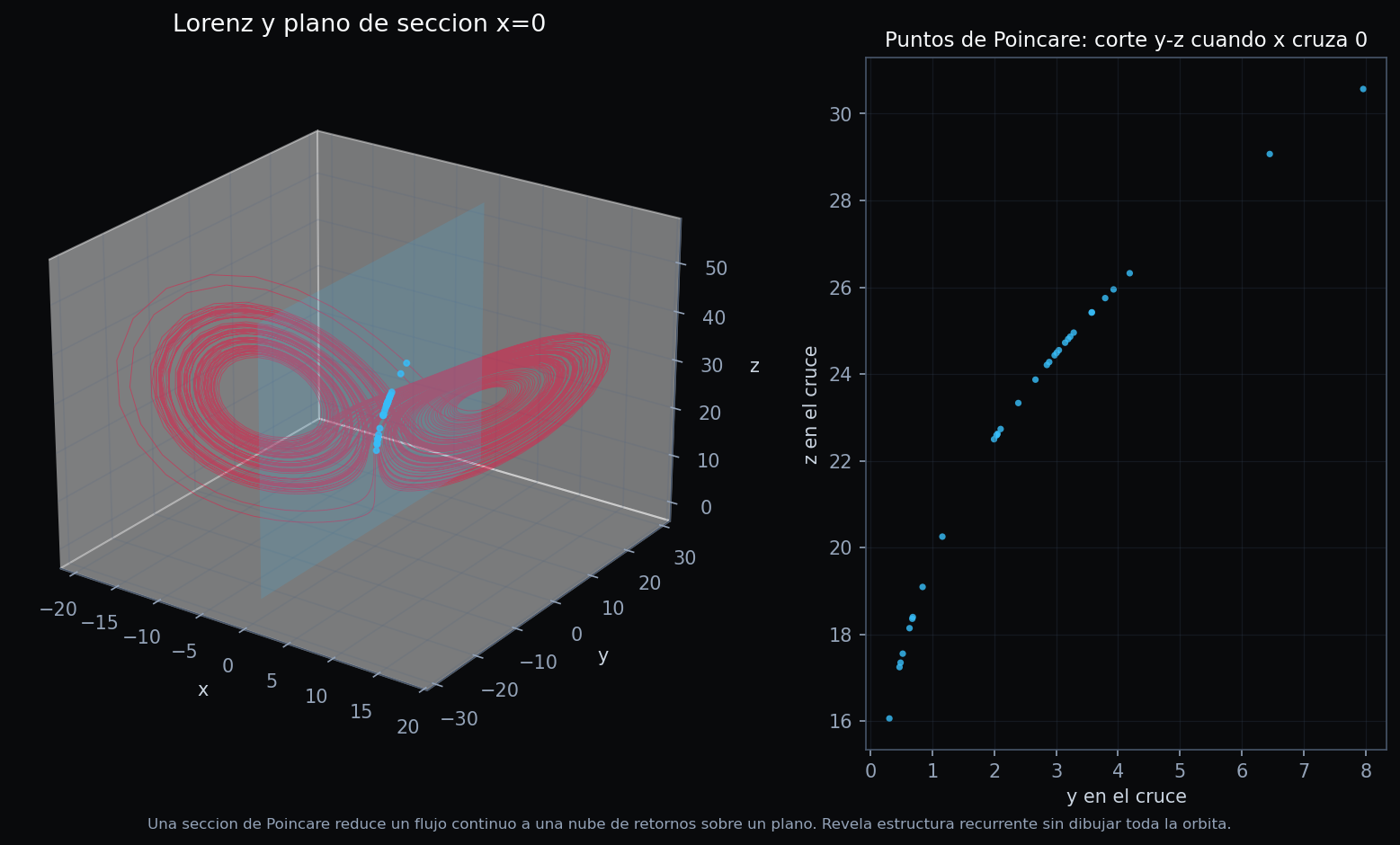
For maps, the retained values are direct iterates. For flows, the toolbox needs an event or measurement rule, such as local maxima, final retained states, or a Poincare crossing. That rule matters because it determines which part of the continuous trajectory becomes a plotted point.

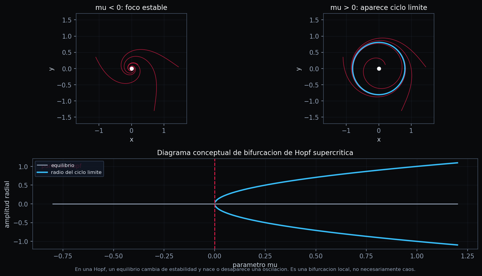
A Hopf bifurcation is a specific local mechanism in which an equilibrium changes stability and an oscillation is born or destroyed. It belongs in the same visual family of parameter-change diagrams, but it should not be confused with a full route to chaos.

How Parameters Change This Figure

Parameter range: too wide can compress important branches; too narrow can hide the route into the behavior you want to show.
Parameter samples: too few samples make the diagram look empty or jagged. Increase density for final plots.
Transient length: too short leaves startup points in the chart. Increase burn-in before interpreting branches.
Retained points: too few retained values hide dense bands; too many values can overplot into a solid block.
Integration step: for flows, a large step can create numerical artifacts that look like bifurcations.
Poincare plane: changing the section plane or crossing direction changes which returns are plotted.